Quantum Gravity

A positivity wedge for inflationary non-Gaussianity

If the inflaton couples to a hidden sector of heavy states, exchange of those states makes the primordial fluctuations non-Gaussian. Unitarity of the hidden sector implies that its two-point function has a spectral decomposition with a non-negative density. De Rham, Jazayeri and Tolley [DJT] used this to show that the shape of the resulting bispectrum is confined to a limited region of shape space. They posed the corresponding question for the quantities experiments report, the amplitudes of the equilateral and orthogonal templates, as a non-linear optimisation problem.

The problem turns out to be linear. Write $\fe$ and $\fo$ for $f_{\rm NL}^{\rm equil}$ and $f_{\rm NL}^{\rm ortho}$, and measure angles in the $(\fe,\fo)$ plane anticlockwise from the positive $\fe$ axis. Under hypotheses (H1)–(H6), stated in sections 1–4 where they are used, the set of reachable $(\fe,\fo)$ is exactly a convex cone, a wedge with its vertex at the origin. Its edges are fixed by two extremal masses and are computed numerically. For the Planck templates and a Planck-like $T{+}E$ bispectrum Fisher metric,

$$164.2^\circ\;\le\;\arg(\fe+i\,\fo)\;\le\;176.2^\circ,$$

so that $\fe<0<\fo$ and $0.067\,\lvert\fe\rvert\le\fo\le0.283\,\lvert\fe\rvert$. Three of the hypotheses carry the result: that the inflaton couples to the hidden sector through a de Sitter-invariant vertex with no boost-breaking admixture (H2), that the three-point function of the hidden sector is negligible (H3), and that the spectral integral needs no subtraction (H4). Without any one of them, positivity no longer implies the wedge. Current measurements are consistent with it: the nearest point of the wedge to each measurement lies at or near the origin, and no dataset excludes the wedge at more than $1.1\sigma$. If the Planck central value persists, CMB-S4 would exclude the wedge at between $2.5\sigma$ and $3.9\sigma$, depending on the assumed sensitivity.

The setting, the positivity argument for the shape and the template question are due to [DJT]. Cabass et al. [Cabass et al. 2024] projected exchange shapes at fixed masses onto the same templates; the single-exchange curve used here coincides with theirs restricted to the de Sitter-invariant ratio of couplings. We add the reduction to a convex cone, the explicit wedge for several noise models, an account of which hypotheses carry it, and the comparison with data.

Familiarity with the primordial bispectrum and its shape function, and with the mass parameter of a field in de Sitter space, is assumed.

1. What is measured

Let $\zeta$ be the curvature perturbation and $B_\zeta(k_1,k_2,k_3)$ its bispectrum. The shape function $S(k_1,k_2,k_3)=(k_1k_2k_3)^2B_\zeta$ is scale invariant in the cases considered here, so it is a function on triangle shapes. A template $S_T$ is a fixed reference shape, normalised so that $S_T(1,1,1)=1$. We use the two Planck templates: the equilateral template of Creminelli et al. and the orthogonal template of Senatore, Smith and Zaldarriaga [SSZ]. The sign convention is that of WMAP and Planck, $f_{\rm NL}\propto+B_\zeta(k,k,k)$. The wedge depends only on the ratio $\fo/\fe$; the comparison with data in section 6 uses Planck’s normalisation of $f_{\rm NL}$.

Experiments fit both templates simultaneously. Given a positive inner product $\langle\cdot,\cdot\rangle$ on shapes, the reported amplitudes of a shape $S$ are the joint least-squares coefficients

$$f=G^{-1}b,\qquad G_{XY}=\langle S_X,S_Y\rangle,\qquad b_X=\langle S,S_X\rangle, \tag{1}$$

with $X,Y\in\{\text{equil},\text{ortho}\}$. We take (1) as the definition of the reported amplitudes (H6). The inner product reflects the experiment’s noise. For the CMB it is the bispectrum Fisher matrix. A common proxy, due to Fergusson and Shellard, is

$$\langle A,B\rangle=\int_{V}A\,B\,\frac{dk_1\,dk_2\,dk_3}{k_1+k_2+k_3},$$

where $V$, the tetrapyd, is the set of $(k_1,k_2,k_3)$ that satisfy the triangle inequalities with each $k_i\le k_{\max}$.

The only property of (1) used below is that $f$ is linear in $S$.

2. Exchange of a hidden sector

Let the hidden sector couple to the inflaton through a scalar operator $\cO$ with $\langle\cO\rangle=0$. We assume (H1) that in the Bunch–Davies state its two-point function has the de Sitter-invariant Källén–Lehmann representation

$$\langle\cO\,\cO\rangle=\int_0^\infty d\mu\;\rho(\mu)\,G(\sigma;\mu),\qquad\rho(\mu)\ge0, \tag{2}$$

where $G(\sigma;\mu)$ is the propagator of a free scalar of mass $m$, $\mu=\sqrt{m^2/H^2-9/4}$, and $\sigma$ is the de Sitter-invariant distance. Positivity of $\rho$ follows from unitarity of the hidden sector. A single free heavy field corresponds to a delta function in $\rho$; a conformal sector, to a power law.

We take (H2) the inflaton to be canonical, with sound speed $c_s=1$, and its coupling to the hidden sector to be $-(\alpha/\Lambda)\sqrt{-g}\,(\partial\phi)^2\cO$, which is invariant under the de Sitter isometries. On the inflating background $\bar\phi(t)$ this coupling produces two vertices, a quadratic one, $-(\alpha/\Lambda)(\partial\delta\phi)^2\cO$, and a linear one, $(2\alpha\dot{\bar\phi}/\Lambda)\,\delta\dot\phi\,\cO$. We assume (H3) that the tree diagram in which $\cO$ is exchanged between these two vertices dominates the bispectrum, so that the three-point function of $\cO$, multiple exchanges and loops can be neglected.

The tree diagram is linear in the in-in propagators of $\cO$, each of which is given by the same spectral integral as (2) [DJT]. The bispectrum is a positive superposition of single exchanges,

$$B(k)=\int_0^\infty d\mu\;\rho(\mu)\,B(k;\mu), \tag{3}$$

where $B(k;\mu)$ is the bispectrum produced by exchanging one free scalar of parameter $\mu$ through the same two vertices.

Equation (3) already indicates why $\fe$ should be negative. The two vertices each carry one power of $\alpha$, so every mass enters with weight $\alpha^2\rho(\mu)\ge0$, and each single exchange is negative at the equilateral point, $B(1,1,1;\mu)<0$ [DJT]. The same observation shows which additions can spoil the result: any contribution odd in a coupling, such as one proportional to $\alpha^3\langle\cO\cO\cO\rangle$, has no definite sign.

3. The cone

At large mass the single-exchange bispectrum decays as $B(k;\mu)\sim\mu^{-2}$: integrating out a heavy field leaves a contact interaction suppressed by $1/m^2$ [DJT]. We assume (H4)

$$\int^\infty d\mu\;\rho(\mu)\,\mu^{-2}<\infty, \tag{4}$$

so that (3) converges without a subtraction. A subtraction would introduce a contact counterterm of arbitrary sign (section 5).

When (1) is applied to (3), dominated convergence lets the linear map pass inside the integral:

$$(\fe,\fo)[\rho]=\int_0^\infty d\mu\;\rho(\mu)\,v(\mu),\qquad v(\mu)\equiv G^{-1}b\big(S(\cdot\,;\mu)\big). \tag{5}$$

The reachable set, as $\rho$ ranges over non-negative densities satisfying (4), is the convex cone generated by the vectors $v(\mu)$. As $\mu\to\infty$, $v(\mu)\to0$ but $\mu^2v(\mu)$ tends to a non-zero vector $v_c$, the projection of the heavy-mass contact shape. Rescaling generators by positive factors does not change the cone, so it is generated equally well by the directions of $v(\mu)$ for $\mu<\infty$, and its closure contains the ray through $v_c$. In two dimensions a closed convex cone is a sector, determined by its two extreme directions.

Lemma (planar cone). Let $\{u_t\}$ be a family of non-zero vectors in $\mathbb R^2$, depending continuously on a parameter $t$ in a closed interval, whose directions lie in a closed arc of opening less than $\pi$. Let $\theta_-$ and $\theta_+$ be the smallest and largest of their angles. Then the closed convex cone generated by the $u_t$ is the sector $\{re^{i\theta}:r\ge0,\ \theta_-\le\theta\le\theta_+\}$.

Proof. The vectors lie in an open half-plane, on which the angle is single-valued, and a positive combination of two vectors less than $\pi$ apart lies angularly between them. Every positive combination thus has its angle in $[\theta_-,\theta_+]$. Conversely, any angle strictly between $\theta_-$ and $\theta_+$ is a positive combination of two of the vectors on either side of it, and the edges are attained by the vectors themselves.

The lemma applies with $u_t$ the unit vectors along $v(\mu)$, parametrised so that $\mu\in[0,\infty]$ maps to a closed interval with the endpoint direction $v_c/\lvert v_c\rvert$; the condition on the opening is verified in section 4. The question of [DJT], which values of the template amplitudes positivity allows, thus reduces to finding the two extreme angles of one curve.

4. The single-exchange curve and the wedge

We assume (H5) that $\rho$ is supported on the principal series, $m\ge3H/2$, so that $\mu$ is real and non-negative. Unitarity also allows lighter states; their effect is treated in section 5.

The single-exchange shape is obtained from the closed-form seed function of [DJT] (their eq. 28), $F(u)$ with $u=k_3/(k_1+k_2)$ in the channel where the exchanged momentum is $k_3$. The seed is the exchange four-point function evaluated at a boundary point of its kinematic space; a differential operator (their eq. 27) converts it into the bispectrum for the two vertices above, and the three channels are summed. Readers who wish to skip these details may treat $v(\mu)$ as numerical input. The seed obeys the boundary differential equation

$$u^2(1-u^2)F''-2u^3F'+\big(\mu^2+\tfrac14\big)F=\frac{u}{1+u}.$$

Numerically, the seed satisfies this equation to $10^{-16}$, matches a series expansion about the folded configuration $u=1$, and agrees with a direct in-in evaluation to between 0.1% and 0.8%. In the limit $\mu\to\infty$ the shape reproduces the contact shape of [DJT] (their eq. 7), and $B(1,1,1;\mu)<0$ for every $\mu$.

We evaluate the curve at 33 masses between $\mu=0.02$ and $\mu=20$, and in the limit $\mu\to\infty$. Below $\mu\approx0.1$ the angle changes by less than $0.1^\circ$, and we take the value at $\mu=0$ to be its limit; the lower edge is then attained by a spectral weight concentrated at $m=3H/2$. Along the curve, the angle $\theta(\mu)=\arg v(\mu)$ increases from its value as $\mu\to0$ to a single maximum at $\mu^\ast\approx2.4$, and then decreases towards the contact direction, which lies strictly inside. The lower edge of the wedge is set by the lightest allowed state, $m=3H/2$, and the upper edge by an intermediate mass. Independent calculations agree on both edges to $0.003^\circ$ and on the sign of the bispectrum. All directions lie in the second quadrant, within an arc of $12.5^\circ$, so the lemma applies.

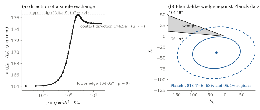
Figure 1. (a) Direction of a single exchange as a function of the mass parameter, for the Fergusson–Shellard inner product. (b) The wedge for the Planck-like $T{+}E$ metric in the $(\fe,\fo)$ plane, with the Planck 2018 $T{+}E$ measurement for comparison (section 6). Angles increase anticlockwise, so the steeper ray is the lower edge. The contours are the two-parameter $\Delta\chi^2=2.30$ and $6.18$ regions.

The edges depend on the inner product as follows.

inner product	lower edge ($\mu\to0$)	upper edge	$\mu^\ast$	contact direction
Fergusson–Shellard proxy	164.05°	176.50°	2.40	174.94°
Planck-like $T{+}E$, $\ell\le2000$	164.19°	176.19°	2.44	174.77°
Planck-like $T$ only	164.23°	176.30°	2.42	174.82°
$T{+}E$, $\ell_{\max}=1500$	164.19°	176.22°	2.44	174.79°
cosmic-variance-limited $T{+}E$, $\ell\le2000$	164.14°	176.40°	2.40	175.00°

The Planck-like metric is the full-sky bispectrum Fisher matrix computed from CAMB transfer functions with Planck-like noise ($33\,\mu$K-arcmin in temperature, $70\,\mu$K-arcmin in polarisation, a 7′ beam and $f_{\rm sky}=0.76$), with the shapes expanded in up to 816 separable basis functions. It gives $\sigma(\fe,\fo)=(53,27)$ for $T{+}E$, compared with Planck’s $(47,24)$. Its matrix mapping effective-field-theory operators to template amplitudes ($T$ only) agrees with that of Planck 2013 [Planck 2013] entry by entry to within 3%; the 2013 version is used for this comparison because the corresponding 2018 formula contains a transcription error (appendix).

Two regularised choices of the modal basis give edges that agree to $0.03^\circ$ (unregularised low-order bases are numerically unstable). The spread in the table reflects the noise model, $\ell_{\max}$ and the choice of $T$ or $T{+}E$. In the Fisher metric the cosine between the two templates, $G_{\rm eo}/\sqrt{G_{\rm ee}G_{\rm oo}}$, is $-0.094$, so that the estimated amplitudes have correlation $+0.094$ (section 6). In the Fergusson–Shellard proxy the cosine is $+0.14$, of the opposite sign; the proxy is a stand-in for a CMB metric, although its edges agree with the Planck-like ones to about $0.3^\circ$.

Galaxy surveys use an orthogonal template adapted to large-scale structure [Cabass et al. 2022]. With a tree-level galaxy-bispectrum Fisher metric at BOSS-like settings ($z=0.57$, linear bias 2, $0.01\le k\le0.08\,h\,{\rm Mpc}^{-1}$), the wedge for that template is $171.0^\circ$–$177.4^\circ$. The upper edge is stable to $0.1^\circ$. Marginalising over the tree-level bias and shot-noise terms moves the lower edge down to about $167^\circ$. With the Planck orthogonal template instead, the marginalised upper edge crosses $180^\circ$, so the sign of $\fo$ in galaxy surveys depends on the template.

5. Which hypotheses carry the wedge

The results of this section are computed with the Fergusson–Shellard inner product, except where stated.

Lighter states. Unitarity allows spectral weight on the complementary series, $0<m^2<9H^2/4$, where $\mu=i\nu$ with $0<\nu<3/2$. The seed continues smoothly to this range, and the angle decreases monotonically as the mass decreases, so only the lower edge moves:

lightest mass $m^2/H^2$	9/4	2.01	1.27	0.56	→ 0
lower edge	164.05°	162.25°	155.57°	147.64°	140.6°

Near the light end the shapes are enhanced in the squeezed limit, and the edge depends strongly on the inner product; with a flat-sky weight proportional to the inverse triangle area it falls to $112.5^\circ$. In every inner product examined the signs $\fe<0<\fo$ are preserved, and the upper edge is unchanged.

A subtraction. If (4) fails and the spectral integral requires one subtraction, a contact term with a coefficient of either sign appears, and the reachable set becomes the cone together with the full line through $v_c$. A set of generators whose consecutive angular gaps are all smaller than $180^\circ$ spans the plane. The generators $176.50^\circ$, $354.94^\circ$ (the negative contact direction) and $164.05^\circ$ leave gaps of $178.4^\circ$ and $169.1^\circ$; for the Planck-like metric the corresponding gaps are $178.6^\circ$ and $169.4^\circ$. Every direction becomes reachable.

The three-point function of $\cO$. The diagram with one $\langle\cO\cO\cO\rangle$ insertion scales as $\alpha^3$, whereas the exchange diagram scales as $\alpha^2$. Changing $\alpha\to-\alpha$ leaves all positivity conditions unchanged and reverses the sign of the $\alpha^3$ term relative to the exchange term, and unitarity does not fix the sign of a three-point function. Once this term is included, positivity no longer implies the wedge. Which directions become reachable depends on the shape of the three-point contribution, which is not computed here.

Boost breaking. In the effective field theory of inflation, write the inflaton fluctuation as $\pi$ and work in unitary gauge, where $\delta g^{00}\equiv g^{00}+1=-2\dot\pi-\dot\pi^2+(\partial_i\pi)^2/a^2+\dots$ and hence $(\delta g^{00})^2=4\dot\pi^2+\dots$. The most general coupling to $\cO$ at this order is $c_1\,\delta g^{00}\cO+c_2(\delta g^{00})^2\cO$. Since $(\partial\phi)^2=\dot{\bar\phi}^2g^{00}$ in unitary gauge, the de Sitter-invariant coupling of section 2 is linear in $\delta g^{00}$ and has $c_2=0$. In general, the coefficient of the $\dot\pi^2\cO$ vertex is $-c_1+4c_2=-c_1(1+\varepsilon_{\rm bb})$, where

$$\varepsilon_{\rm bb}\equiv-4c_2/c_1$$

measures the boost-breaking admixture (it is unrelated to the slow-roll parameter). The linear vertex $\dot\pi\,\cO$ is common to all exchange diagrams; the quadratic vertex splits into a $\dot\pi^2\cO$ part and an $(\partial_i\pi)^2\cO$ part, whose exchange shapes we denote $S^{(t)}_\mu$ and $S^{(s)}_\mu$. The exchange then becomes $c_1^2\int\rho\,\big[S^{(s)}_\mu+(1+\varepsilon_{\rm bb})S^{(t)}_\mu\big]$. A de Sitter-invariant higher operator such as $((\partial\phi)^2)^2\cO$ contributes to $c_2$ on the rolling background, giving $\varepsilon_{\rm bb}\sim\dot{\bar\phi}^2/\Lambda^4$ of either sign. That this admixture can reverse the sign of the equilateral bispectrum was shown by Ghosh, Maity and Ullah [GMU].

For each fixed $\varepsilon_{\rm bb}$ the reachable set is again a cone. The following table lists the union of these cones over a range of $\varepsilon_{\rm bb}$; a union of cones need not be convex.

range of $\varepsilon_{\rm bb}$	reachable $\arg(\fe+i\fo)$
$\varepsilon_{\rm bb}=0$	164.05°–176.50°
$\lvert\varepsilon_{\rm bb}\rvert\le0.35$	163.90°–177.20°
$\lvert\varepsilon_{\rm bb}\rvert\le1.25$	163.50°–179.89°
$\varepsilon_{\rm bb}\ge0$	all directions except 176.55°–352.4°
$\varepsilon_{\rm bb}\le0$, or unrestricted	all directions

For a single operator with constant $\varepsilon_{\rm bb}$, the last row rests on the range $-40\lesssim\varepsilon_{\rm bb}\lesssim-11$, where the generator directions span an arc wider than $180^\circ$ by less than $1^\circ$, so that the cone for that single value is already the whole plane. With two operators, $\varepsilon_{\rm bb}$ can vary with $\mu$, and the row holds without relying on that narrow margin. The quadrant $\fe<0<\fo$ is preserved exactly when $-1.277<\varepsilon_{\rm bb}<19.75$. The question is whether some principle fixes the sign of $\varepsilon_{\rm bb}$.

Claim. Spectral positivity (including its matrix form for several operators) and the reflection and propagator positivity conditions of Lee and Melville [Lee–Melville] do not fix the sign of $\varepsilon_{\rm bb}$.

Argument. Each of these conditions is a consequence of the positivity of the spectral density (or of the spectral matrix) of the hidden sector, and it holds for any real values of the vertex coefficients $c_1,c_2$. None of them can constrain the ratio $\varepsilon_{\rm bb}=-4c_2/c_1$: explicit parameter points of either sign satisfy all of them. With two operators $\cO_1,\cO_2$, the cross spectral density $\rho_{12}$ is constrained only by $\lvert\rho_{12}\rvert\le\sqrt{\rho_{11}\rho_{22}}$, which leaves the sign of the effective $\varepsilon_{\rm bb}$ free at each $\mu$. Perturbative unitarity bounds the magnitude of $c_2$ relative to the cutoff of the effective theory, but is insensitive to its sign. The argument covers the conditions listed; it does not exclude a principle that constrains the vertex coefficients directly.

Boost-breaking $2\to2$ positivity [Grall–Melville] is sensitive to the sign of $c_1c_2$. For a single heavy $\cO$ that accounts for the whole quartic self-interaction of $\pi$, their condition must hold for every value $\gamma\ge1$ of their kinematic parameter within the validity of the effective theory. At $\gamma=1$ it excludes $-7.65<\varepsilon_{\rm bb}<-0.349$; the excluded interval scales as $1/\gamma$, so the full condition excludes at least this interval. Adding one further state coupled only through $(\delta g^{00})^2$ removes the exclusion for every $\gamma$, so in general the condition constrains the quartic interaction and not $\varepsilon_{\rm bb}$.

In one class the sign is fixed, and $\varepsilon_{\rm bb}=0$ becomes equivalent to $c_s=1$.

Proposition ($P(X)\cdot\cO$ class). Suppose $\cO$ multiplies the full kinetic function of the inflaton, $\mathcal L\supset P(X)\,\cO/M$ with $X=-\tfrac12(\partial\phi)^2$ and $M$ a constant. Then $\varepsilon_{\rm bb}=2X_0P_{XX}/P_X=c_s^{-2}-1\ge0$, with equality if and only if $c_s=1$.

Proof. In unitary gauge $X=X_0(1-\delta g^{00})$. Expanding $P$ to second order in $\delta g^{00}$ gives $c_1=-X_0P_X/M$ and $c_2=\tfrac12X_0^2P_{XX}/M$, so $\varepsilon_{\rm bb}=-4c_2/c_1=2X_0P_{XX}/P_X$. The sound speed of a $P(X)$ theory is $c_s^2=P_X/(P_X+2X_0P_{XX})$, hence $\varepsilon_{\rm bb}=c_s^{-2}-1$. The sign follows from $P_X>0$, required for the absence of ghosts, together with the assumption $P_{XX}\ge0$, equivalent to subluminal propagation, $c_s\le1$.

Within this class, (H2) reduces to the single condition $c_s=1$, under which the wedge holds exactly. We have not computed the exchange shapes for $c_s<1$, so only the sign $\varepsilon_{\rm bb}\ge0$ is established.

6. Comparison with data

The comparison uses published central values and correlations with two degrees of freedom. The direction is the angle of the central value, the correlation is that between the errors on $\fe$ and $\fo$, and the significance is the Gaussian equivalent of the $\chi^2_2$ tail probability at the minimum $\chi^2$ within the wedge.

data	correlation	direction	$\chi^2$ at origin	min $\chi^2$ in wedge
Planck 2018 $T{+}E$: $(-26\pm47,\ -38\pm24)$ [Planck 2018]	+0.094	235.6°	2.67	2.63 (1.1σ)
BOSS, Cabass et al.: $(940\pm600,\ -170\pm170)$ [Cabass et al. 2022]	−0.40	349.7°	2.62	2.62 (1.1σ)
BOSS, D’Amico et al.: $(207\pm292,\ -68\pm73)$ [D’Amico et al.]	−0.23	341.8°	1.13	1.13 (0.6σ)

The Planck correlation is computed from the Fisher matrix of section 4, and the BOSS errors are symmetrised. Planck is compared with the CMB wedge and the BOSS results with the galaxy-survey wedge. For both BOSS results the nearest wedge point is the origin, so the marginalised and unmarginalised variants of that wedge give the same result; for Planck it is $(-9.2,\,0.6)$, about 9 units from the origin. All three central values lie outside the wedge, and the comparison amounts to a test of consistency with zero non-Gaussianity, which all three pass.

Excluding the wedge at $3\sigma$ likewise amounts to detecting non-Gaussianity at $3\sigma$ in a direction outside it. With the Planck central value and correlation held fixed, this requires $\sigma(\fe,\fo)\le(22,11)$ ($\Delta\chi^2=11.83$ for two degrees of freedom), approximately half the current uncertainties. The forecasts below combine each experiment’s published uncertainties with the correlation $+0.094$ and the Planck central value. For MegaMapper, the Planck central value is mapped to galaxy-survey template coordinates through the effective-field-theory operators, giving $(-36.5,\,-24.3)$; those rows are illustrative.

experiment	$\sigma(\fe,\fo)$	wedge	exclusion if the Planck central value persists
Simons Observatory, baseline / goal [SO]	(27, 14) / (24, 13)	CMB	2.3σ / 2.5σ
CMB-S4, published forecast [S4]	(21.2, 9.1)	CMB	3.9σ
CMB-S4-like, Fisher matrix of section 4 ($T{+}E$, $\ell\le2500$)	(27, 13)	CMB	2.5σ
MegaMapper, conservative [MegaMapper]	(23, 12)	galaxy	1.7σ
MegaMapper and CMB-S4 combined	(14, 7)	galaxy	3.3–3.4σ

The wedge is falsified by a $3\sigma$ detection with $\fe>0$ or $\fo<0$, or with a direction outside $164.2^\circ$–$176.2^\circ$ for the CMB templates.

7. Discussion

The wedge is a property of a model class. Within that class the cone is exact, and the edge angles are numerical, with a dependence on the noise model of a few tenths of a degree for the CMB and a few degrees for galaxy surveys. A subtraction, a non-negligible three-point function of $\cO$, or a boost-breaking admixture of unrestricted sign would each remove the wedge. The lower edge follows from the assumed gap $m\ge3H/2$, not from unitarity; lighter states lower it to about $141^\circ$ for the Fergusson–Shellard inner product, and further for others. The cone constrains the direction of $(\fe,\fo)$ but not its magnitude.

The comparison of section 6 uses Fisher-matrix inner products. The CMB metric omits ISW–lensing and foreground contributions, uses approximate Planck noise and neglects the spectral tilt in the templates, each estimated to shift the edges by less than $0.1^\circ$. The galaxy-survey metric is a tree-level Gaussian Fisher matrix, not the one-loop BOSS likelihood. For parameter inference a full-likelihood analysis of the exchange shapes is preferable; the wedge is a statement about the template amplitudes that experiments report.

It remains open whether any principle constrains the vertex coefficients, and hence the sign of $\varepsilon_{\rm bb}$; how the wedge changes for exchange at sound speed $c_s<1$ outside the $P(X)$ class; and which shapes the three-point function of a unitary hidden sector can take.

Appendix: the Planck 2018 conversion formula

Planck 2018 IX [Planck 2018], eq. (58), gives the map from the effective-field-theory parameters $(c_s,\tilde c_3)$ to $(\fe,\fo)$. With $\beta=(1-c_s^2)/c_s^2$ it reads

$$\fe=\beta\big[-0.275-0.0780\,c_s^2-\tfrac23\times0.780\,\tilde c_3\big],\qquad \fo=\beta\big[0.0159-0.0167\,c_s^2-\tfrac23\times0.0167\,\tilde c_3\big].$$

To check it, write each amplitude as $f_X=a_X\,f^{\dot\pi(\partial\pi)^2}+b_X\,f^{\dot\pi^3}$, where the two operator amplitudes are $f^{\dot\pi(\partial\pi)^2}=-\tfrac{85}{324}\beta$ and $f^{\dot\pi^3}=-\tfrac{10}{243}\beta\big(\tilde c_3+\tfrac32c_s^2\big)$. The coefficient $b_X$ appears twice in each row, once multiplying $c_s^2$ and once multiplying $\tilde c_3$, and the two occurrences must agree.

In the equilateral row the $c_s^2$ term gives $b_{\rm eq}=1.264$, whereas the $\tilde c_3$ term gives $12.64$. The row is consistent only if $0.780$ is read as $0.0780$. The orthogonal row is internally consistent, with $b_{\rm or}=+0.2705$. Planck 2013 XXIV [Planck 2013], eq. (98), writes, with the same prefactor $\beta$, $\fo=\beta(0.0159-0.0167A)$ with $A=-(c_s^2+\tfrac23\tilde c_3)$. Expanding gives $\fo=\beta\big(0.0159+0.0167\,c_s^2+\tfrac23\times0.0167\,\tilde c_3\big)$, that is, $b_{\rm or}=-0.2705$, which agrees in sign with Senatore, Smith and Zaldarriaga [SSZ], eq. (102), and with the Fisher matrix of section 4 ($-0.2676$). The 2015 paper [Planck 2015], eq. (87), appears to have expanded the 2013 formula with both orthogonal terms reversed in sign and the leading zero of $0.0780$ omitted, and the 2018 paper reproduces it. The corrected orthogonal row is

$$\fo=\beta\big[0.0159+0.0167\,c_s^2+\tfrac23\times0.0167\,\tilde c_3\big].$$

Inverting the Planck 2018 central values with the 2013 coefficients gives $c_s=0.031$, the value quoted by Grall and Melville [Grall–Melville], whereas the printed 2018 coefficients give $c_s^2<0$. This suggests that the error is confined to the printed equation. The projections in this note compute $(\fe,\fo)$ directly from the shapes and do not use eq. (58).

References

1. de Rham, Jazayeri, Tolley, “Bispectrum islands,” arXiv:2506.19198.
2. Senatore, Smith, Zaldarriaga, “Non-Gaussianities in single field inflation and their optimal limits from the WMAP 5-year data,” arXiv:0905.3746.
3. Cabass, Ivanov, Philcox, Simonović, Zaldarriaga, arXiv:2201.07238.
4. D’Amico, Lewandowski, Senatore, Zhang, arXiv:2201.11518.
5. Cabass, Philcox, Ivanov et al., “BOSS constraints on massive particles during inflation: the cosmological collider in action,” arXiv:2404.01894.
6. Grall, Melville, “Positivity bounds without boosts,” arXiv:2102.05683.
7. Lee, Melville, “Propagator positivity bounds for cosmological correlators,” arXiv:2512.20706.
8. Ghosh, Maity, Ullah, “Massive exchange and the sign of the equilateral bispectrum,” arXiv:2604.06145.
9. Planck Collaboration, “Planck 2013 results. XXIV. Constraints on primordial non-Gaussianity,” arXiv:1303.5084.
10. Planck Collaboration, “Planck 2015 results. XVII. Constraints on primordial non-Gaussianity,” arXiv:1502.01592.
11. Planck Collaboration, “Planck 2018 results. IX. Constraints on primordial non-Gaussianity,” arXiv:1905.05697.
12. Simons Observatory Collaboration, “The Simons Observatory: science goals and forecasts,” arXiv:1808.07445.
13. CMB-S4 Collaboration, “CMB-S4 science book, first edition,” arXiv:1610.02743.
14. Cabass, Ivanov, Philcox et al., “Constraining single-field inflation with MegaMapper,” arXiv:2211.14899.