Quantum Gravity

The low multipoles of holographic cosmology at large flavour number

In holographic cosmology the primordial power spectrum is computed from the stress-tensor two-point function of a three-dimensional SU($N$) gauge theory with many scalar and fermion fields. The published two-loop form fits the Planck temperature spectrum at multipoles $\ell\ge30$, but it is not valid at lower $\ell$, which were therefore excluded from the fits. We ask what the same theory predicts for $\ell<30$. When all scalars are conformally coupled and quartic and Yukawa couplings are negligible, the answer is fixed at leading order in the number of fields: the gauge-field contribution to the trace correlator, with both gluon lines dressed by the chain of matter loops, can be computed exactly. Its expansion reproduces the published two-loop coefficient $64/(3\pi^2)$, and below a crossover scale, corresponding to $\ell_c\approx3$–$4$ for the fitted parameters, the logarithm that drives the two-loop running stops growing. The low-$\ell$ spectrum then follows from the three parameters already fitted at $\ell\ge30$, with no new parameter.

Positivity of the power spectrum at all scales bounds $N_B=1+\sum_M(1-8\xi_M)^2$, which counts the gauge field plus the non-conformally coupled scalars weighted by $(1-8\xi_M)^2$, by $N_B\le0.864\,\beta$, where $\beta$ is one of the fitted parameters. The bound assumes two properties of the resummed correlator that we establish numerically, and for $N_B>1$ it holds within a model that extends the calculation to that case. Over the published one-standard-deviation ranges of $\beta$ it gives $N_B\lesssim1.6$–$2.9$, which excludes the explicit solution with $N_B\approx88$ given with the model. Fitted to Planck temperature data at all multipoles, with a compressed likelihood, the resummed spectrum is worse than $\Lambda$CDM by $\Delta(-2\ln\mathcal L)\approx3$–$5$, depending on the treatment of the background cosmology, and predicts a quadrupole $0.57$ times the $\Lambda$CDM value.

The framework is due to McFadden and Skenderis [MS 2009], [MS 2010]. Afshordi, Corianò, Delle Rose, Gould and Skenderis [ACDGS] reported the two-loop coefficients, whose computation Corianò, Delle Rose and Skenderis later gave in full [CDS], and fitted the model to Planck 2015 data; they found the fit at all multipoles disfavoured relative to $\Lambda$CDM with running, and attributed this to the breakdown of perturbation theory at $\ell\lesssim30$. Afshordi, Gould and Skenderis [AGS] repeated the analysis in more detail. The dressing of a three-dimensional gauge field by a large number of matter fields is standard; at the resulting infrared fixed point, Giombi, Tarnopolsky and Klebanov [GTK] compute the stress-tensor two-point coefficient of conformal QED to next-to-leading order in $1/N$. What is new here is the crossover of the trace correlator between the perturbative and infrared regimes, together with its consequences for the low-$\ell$ spectrum, for positivity and for the fit to data.

Familiarity with the holographic cosmology dictionary is not assumed beyond eq. (1) below; familiarity with one-loop computations in three-dimensional gauge theory and with CMB power spectra is.

1. The two-loop spectrum and where it fails

The dual theory is SU($N$) Yang–Mills theory in three Euclidean dimensions coupled to $N_\Phi$ real scalars and $N_\psi$ two-component Dirac fermions, all in the adjoint representation [ACDGS]. Scalars couple to the background curvature with parameters $\xi_M$; the value $\xi_M=1/8$ is conformal coupling in three dimensions. The theory is super-renormalizable, and its dimensionless coupling at momentum $q$ is the ‘t Hooft coupling $\lambda=g_{\rm YM}^2N/q$.

The trace $\Theta=T^i{}_i$ of the stress tensor carries the scalar perturbations. At large $N$ its two-point function has the form $\langle\Theta(q)\Theta(-q)\rangle=N^2q^3f(\lambda)$ up to local terms, and the holographic dictionary [MS 2009], in the form used in [ACDGS] and [CDS], gives the curvature power spectrum

$$\Delta^2(q)=\frac{1}{4\pi^2N^2f(\lambda)}. \tag{1}$$

The dictionary involves the analytic continuation $q\to-iq$, $N\to-iN$, which leaves $\lambda$ and $f$ unchanged [CDS], so $\lambda>0$ throughout. In perturbation theory [ACDGS], [CDS],

$$f(\lambda)=f_0\big[1-f_1\lambda\ln\lambda+f_2\lambda+O(\lambda^2)\big],\qquad f_0=\frac{N_B}{64},\qquad N_B=1+\sum_M(1-8\xi_M)^2. \tag{2}$$

The “1” in $N_B$ is the gauge field; each scalar contributes $(1-8\xi_M)^2$, which vanishes for conformal coupling, and fermions do not contribute to $f_0$. With all $\xi_M=1/8$ and no Yukawa couplings, eq. (8) of [ACDGS] gives

$$f_1=-\frac{4}{3\pi^2}\Big(N_\psi+\frac{N_\Phi}{2}-2\Big),\qquad N_B=1.$$

Writing $gq_\ast=f_1g_{\rm YM}^2N$ and $\ln(1/\beta)=f_2/f_1+\ln\lvert f_1\rvert$, with the pivot $q_\ast=0.05\,{\rm Mpc}^{-1}$, and expanding $1/f$ to first order, (1) becomes the form used in the fits [ACDGS],

$$\Delta^2(q)=\frac{\Delta_0^2}{1+u\ln u+u\ln\beta},\qquad u\equiv\frac{\lvert g\rvert q_\ast}{q},\qquad\Delta_0^2=\frac{1}{4\pi^2N^2f_0}. \tag{3}$$

The fits find $g<0$, which requires $f_1<0$; the variable $u=\lambda\lvert f_1\rvert$ is positive. The three parameters $(\Delta_0^2,g,\ln\beta)$ replace the amplitude and tilt of $\Lambda$CDM. Fitted to Planck 2015 data at $\ell\ge30$, [ACDGS] (Table 1) find $g=-0.0131^{+0.0045}_{-0.0035}$ and $\ln\beta=1.01^{+0.21}_{-0.27}$; the fit at all multipoles gives $g=-0.0070^{+0.0011}_{-0.0017}$ and $\ln\beta=0.88^{+0.19}_{-0.24}$.

Multipoles and wavenumbers are related by $\ell\approx q\chi_\ast$, with $\chi_\ast=13\,873$ Mpc the comoving distance to last scattering in the Planck 2018 cosmology. At the quadrupole, the $\ell\ge30$ fit has $u\approx4.5$, so (3) is outside its range of validity. Extrapolated anyway, it predicts a quadrupole $0.32$ times the $\Lambda$CDM value, and with the compressed likelihood of section 6 it worsens the fit at $\ell<30$ by $\Delta(-2\ln\mathcal L)\approx+24$.

2. The expansion parameter is the number of fields

The two-loop term in (2) is large at low $\ell$ although the ‘t Hooft coupling there is small. The tensor-to-scalar ratio of the model is $r=32N_B/N_A$ with $N_A=1+2N_\psi+N_\Phi$ [ACDGS], so the bound $r<0.036$ [BK18] requires $N_A>889$ when $N_B=1$. Since $N_\psi+N_\Phi/2=(N_A-1)/2$, the coefficient above is

$$\lvert f_1\rvert=\frac{2}{3\pi^2}(N_A-5)\gtrsim60,$$

and $\lambda=u/\lvert f_1\rvert\le0.1$ at $\ell=2$ for every parameter set used in this note. The two-loop correction is not small because $f_1$ counts all the matter fields, while $f_0$ counts only the gauge field.

Each matter field contributes to the one-loop vacuum polarisation of the gluon, and this fixes the relevant limit. In three dimensions a massless two-component fermion of unit charge gives a self-energy $e^2k/16$ and a complex scalar the same, so that a real adjoint scalar contributes $g_{\rm YM}^2Nk/32$ and an adjoint fermion $g_{\rm YM}^2Nk/16$ (the adjoint index factor is $N$). Summing the chain of these bubbles gives the dressed gluon propagator, in a normalisation where the free propagator is $1/k^2$,

$$D(k)=\frac{1}{k^2+q_ck},\qquad q_c=g_{\rm YM}^2N\Big(\frac{N_\Phi}{32}+\frac{N_\psi}{16}\Big)=g_{\rm YM}^2N\,\frac{N_A-1}{32}. \tag{4}$$

Each bubble is suppressed by $g_{\rm YM}^2$ and enhanced by the number of fields, so at fixed $q_c$ the bubble chain is leading order in $1/N_A$. The ratio of the three-loop term in which one bubble is inserted into the two-loop diagram to the two-loop term itself is of order $q_c/q$. We therefore expand in $1/N_A$ at fixed

$$x\equiv\frac{q_c}{q}=\kappa u,\qquad\kappa=\frac{q_c}{\lvert g\rvert q_\ast}=\frac{(N_A-1)/32}{\lvert f_1\rvert}=\frac{3\pi^2}{64}\,\frac{N_A-1}{N_A-5}. \tag{5}$$

The variables in play are the ‘t Hooft coupling $\lambda$, which is small; the two-loop expansion parameter $u=\lvert f_1\rvert\lambda$, which is large at low $\ell$ because $\lvert f_1\rvert\gtrsim60$; and $x=q_c/q$, the variable of the resummation. For $N_A>889$, $\kappa$ equals $3\pi^2/64=0.4626$ to within $0.5\%$, and we use that value. The crossover $x=1$ lies at $\ell_c=\kappa\lvert g\rvert q_\ast\chi_\ast$, which is $4.2$ for the published $\ell\ge30$ value of $g$.

We assume from here on that (A1) all scalars are conformally coupled, $\xi_M=1/8$, so that $N_B=1$; (A2) Yukawa couplings vanish; and (A3) quartic couplings are small enough that their own bubble chains can be neglected. At $\xi_M=1/8$ the quartic couplings drop out of the two-loop $f$ (their contribution to the constant term of eq. (9) of [ACDGS] is proportional to $(8\xi_{M_1}-1)(8\xi_{M_2}-1)$), but a flavour-singlet quartic coupling would generate a chain of scalar bubbles at a scale proportional to $\lambda_{\rm quartic}N_\Phi$ and could alter the low-$\ell$ spectrum; (A3) excludes this.

3. The resummed trace correlator

Under (A1)–(A3) the scalars and fermions are classically conformal, up to the neglected quartic couplings, and the parts of $\Theta$ built from them vanish on the equations of motion; their insertions in correlators produce only contact terms. The trace is then the gauge-field term $\Theta_A=\tfrac14F^a_{\mu\nu}F^a_{\mu\nu}$ (in the normalisation of (4)), whose free two-point function is the “1” in $N_B$. The matter fields enter only through the dressing (4). At leading order in $1/N_A$ the trace correlator is therefore the one-loop diagram of $\Theta_A$ with both gluon lines replaced by $D$.

That no other diagram contributes at this order is a power-counting argument, not a proof: with the propagator (4), each additional gluon exchange or matter loop attached to the two gluon lines costs a factor $g_{\rm YM}^2N/q_c\sim1/N_A$ at every $q$, including $q\ll q_c$, where $D\approx1/(q_ck)$. The pure-gauge two-loop term, the “$-2$” in $f_1$, is of this kind. The counting fails when some scalar has $\xi_M\ne1/8$: then $\Theta$ has a matter part, the mixed correlators $\langle\Theta_\Phi\Theta_A\rangle$ are of the same order as the gauge loop, and they are not included here. This is why the controlled case is $N_B=1$.

The first two terms

The expansion in $q_c$ can be done in closed form and checks the normalisation before the full function is computed.

Proposition 1 (two-loop logarithm). Per colour component (that is, with the factor $N^2$ of section 1 removed), the gauge-field trace correlator with the propagator (4) has, to first order in $q_c$, the non-analytic part

$$\langle\Theta_A\Theta_A\rangle(q)=\frac{q^3}{64}-\frac{q_c\,q^2\ln q}{3\pi^2}+\dots,$$

where the dots stand for terms analytic in $q$ and terms of order $q_c^2$. Equivalently, the ratio $\mathcal F=64\langle\Theta_A\Theta_A\rangle/q^3$ obeys $\mathcal F=1+a_1x\ln x+O(x)$ with $a_1=64/(3\pi^2)$.

Proof. The correlator of $F_{\mu\nu}$ involves only the transverse part of the gluon propagator, so we may use $\langle A_\mu(r)A_\nu(0)\rangle=\delta_{\mu\nu}G(r)$ with $G$ the Fourier transform of $D$. Expanding $D=1/k^2-q_c/k^3+O(q_c^2)$ and transforming,

$$G(r)=\frac{1}{4\pi r}+\frac{q_c}{2\pi^2}\ln r+\text{const}+O(q_c^2),$$

since $\nabla^2\ln r=1/r^2$ and the transform of $1/k$ is $1/(2\pi^2r^2)$; the constant drops out of $F_{\mu\nu}$. Then $\langle F_{\mu\nu}(r)F_{\rho\sigma}(0)\rangle=-(\partial_\mu\partial_\rho G\,\delta_{\nu\sigma}-\partial_\mu\partial_\sigma G\,\delta_{\nu\rho}-\partial_\nu\partial_\rho G\,\delta_{\mu\sigma}+\partial_\nu\partial_\sigma G\,\delta_{\mu\rho})$, and by Wick’s theorem $\langle\Theta_A(r)\Theta_A(0)\rangle=\tfrac18\sum\langle F_{\mu\nu}F_{\rho\sigma}\rangle^2$. Carrying out the sums gives

$$\langle\Theta_A(r)\Theta_A(0)\rangle=\frac{3}{16\pi^2r^6}-\frac{q_c}{2\pi^3r^5}+O(q_c^2).$$

In three dimensions the Fourier transform of $r^{-2a}$ is $\pi^{3/2}2^{3-2a}\Gamma(\tfrac32-a)\Gamma(a)^{-1}q^{2a-3}$. At $a=3$ this is $\pi^2q^3/12$, so the first term gives $q^3/64$. At $a=\tfrac52+\epsilon$ we have $\Gamma(\tfrac32-a)=\Gamma(-1-\epsilon)=1/\epsilon+O(1)$ and $q^{2a-3}=q^2(1+2\epsilon\ln q+\dots)$, so the transform is $\pi^{3/2}2^{-2}\Gamma(\tfrac52)^{-1}q^2(1/\epsilon+2\ln q)+O(\epsilon)=\tfrac{2\pi}{3}q^2\ln q$ plus a local $q^2$ term. The second term therefore gives $-q_cq^2\ln q/(3\pi^2)$ plus a local term. At fixed $q_c$, $x\ln q=x\ln q_c-x\ln x$, and the first piece is analytic in $q$. Dividing by $q^3/64$ gives $a_1=64/(3\pi^2)$.

The free term reproduces the normalisation $f_0=1/64$ per unit of $N_B$. For the logarithm, translate back to (2): with $x=\kappa\lambda\lvert f_1\rvert$ and $N_B=1$, the term $a_1x\ln x$ contributes $-f_1\lambda\ln\lambda$ with $-f_1=a_1(N_\Phi/32+N_\psi/16)=\tfrac{4}{3\pi^2}(N_\psi+N_\Phi/2)$. This is the published coefficient, fermion and scalar terms separately, apart from the pure-gauge $-2$, which is of relative order $1/N_A$ and is not part of the leading order. Since $a_1$ comes from the gauge loop alone and the bubble coefficients $1/16$ and $1/32$ from the one-loop vacuum polarisation, the agreement is an independent check of both. It also shows that at $\xi=1/8$ the entire matter logarithm of the two-loop result comes from the self-energy insertion. The check concerns only the first order in $x$; the low-$\ell$ spectrum depends on $x\gtrsim1$, where the full function is needed.

The contact term

The full calculation produces a term independent of $q$, which in $\mathcal F$ would appear as a multiple of $x^3$ and would dominate at small $q$. It does not enter the power spectrum, which is computed from the spin-0 form factor $\mathcal B(q)$ in the decomposition $\langle T_{ij}T_{kl}\rangle=\mathcal A(q)\Pi_{ijkl}+\mathcal B(q)\pi_{ij}\pi_{kl}$ of the transverse part of the correlator [CDS]. Here $\pi_{ij}=\delta_{ij}-q_iq_j/q^2$ and $\Pi_{ijkl}=\tfrac12(\pi_{ik}\pi_{jl}+\pi_{il}\pi_{jk}-\pi_{ij}\pi_{kl})$; away from contact terms $\langle\Theta\Theta\rangle=4\mathcal B$.

Lemma 1 (no constant in $\mathcal B$). A term in $\langle T_{ij}T_{kl}\rangle$ independent of $q$ does not contribute to $\mathcal B$.

Proof. A term independent of $q$ is local and has no derivatives. By diffeomorphism invariance the only such term in the generating functional is $c\int d^3x\sqrt{\gamma}$, with $\gamma_{ij}$ the background metric of the dual theory, whose second variation at flat space is

$$c\Big[\tfrac14\delta_{ij}\delta_{kl}-\tfrac14(\delta_{ik}\delta_{jl}+\delta_{il}\delta_{jk})\Big].$$

Projecting each index with $\pi$ gives $c\big[\tfrac14\pi_{ij}\pi_{kl}-\tfrac14(\pi_{ik}\pi_{jl}+\pi_{il}\pi_{jk})\big]=-\tfrac{c}{2}\Pi_{ijkl}+0\cdot\pi_{ij}\pi_{kl}$, so its transverse part lies entirely in $\mathcal A$.

The constant is nonetheless present in the full trace $\delta_{ij}\delta_{kl}\langle T_{ij}T_{kl}\rangle$, with weight $\tfrac34c$; it belongs to the Ward identity involving $\langle T_{ij}\rangle$. We therefore remove it, which amounts to $\mathcal B(0)=0$.

The full crossover

The dressed propagator has a positive spectral representation over a mass $m$,

$$D(k)=\int_0^\infty dm\,\frac{\rho(m)}{k^2+m^2},\qquad\rho(m)=\frac{2}{\pi}\,\frac{q_c}{m^2+q_c^2},$$

which reduces the dressed loop to a superposition of loops with two massive vector propagators. The sum over polarisations gives the numerator $4[(k\cdot p)^2+k^2p^2]$ for gluon momenta $k$ and $p=q-k$. Writing $k\cdot p=\tfrac12(q^2-k^2-p^2)$ and setting $k^2=-m_1^2$, $p^2=-m_2^2$ wherever a propagator is not cancelled, the remaining terms have one propagator cancelled and are polynomials in $q$ of degree at most 2. With the three-dimensional bubble $\int\frac{d^3k}{(2\pi)^3}\frac{1}{(k^2+m_1^2)(p^2+m_2^2)}=\frac{\arctan(q/(m_1+m_2))}{4\pi q}$ and the prefactor $\tfrac18$ from Wick’s theorem, $\langle\Theta_A\Theta_A\rangle=\frac{1}{32\pi}\int\!\!\int\rho\rho\,J$; dividing by $q^3/64$,

$$\mathcal F(q)=\frac{2}{\pi q^3}\int_0^\infty\!\!\int_0^\infty dm_1dm_2\,\rho(m_1)\rho(m_2)\Big[J(q)-J_0-q^2J_2\Big],\quad J=\big[(q^2+m_1^2+m_2^2)^2+4m_1^2m_2^2\big]\frac{\arctan\frac{q}{m_1+m_2}}{q}, \tag{6}$$

where $J_0$ and $J_2$ are the coefficients of $q^0$ and $q^2$ in the expansion of $J$ about $q=0$. As $q_c\to0$, $\rho$ tends to a delta function at $m=0$ and $\mathcal F\to1$, which fixes the normalisation; the numerical value of $a_1$ below confirms it independently. The first subtraction implements $\mathcal B(0)=0$. The second removes a local term $\propto q_cq^2$, whose coefficient is a logarithmically divergent renormalisation constant. The integral (6) converges absolutely.

We evaluated (6) by trapezoidal quadrature in $\ln m_1,\ln m_2$, with a series expansion of the subtracted integrand for $q\ll m_1+m_2$; doubling the grid changes $\mathcal F$ by less than $10^{-12}$. At small $x$, a fit gives $\mathcal F=1+a_1x\ln x+b\,x+O(x^2\ln^2x)$ with $a_1$ equal to $64/(3\pi^2)$ to $10^{-6}$, as Proposition 1 requires, and $b=1.98139$, which agrees with $\tfrac{11}{12}a_1$ to at least six significant digits; we have not derived that value. The function decreases monotonically from 1 to 0 and is positive for all $x$, with $\mathcal F=0.920,\ 0.644,\ 0.199,\ 0.026$ at $x=0.01,\ 0.1,\ 1,\ 10$. At large $x$, $\mathcal F\approx0.274/x$, so in this subtraction scheme the large-$x$ expansion has neither a constant nor a term linear in $x$. The disappearance of the constant is expected: for $q\ll q_c$ the gauge field becomes part of the conformal infrared theory of the matter fields, whose trace correlator has no $q^3$ term.

The subtraction scheme in (6) is arbitrary up to a term linear in $x$, since that term is the local counterterm $\propto q_cq^2$; changing the scheme adds the same multiple of $x$ at all $x$. This term will be fixed in section 4 by matching to the measured $\ln\beta$ at high $\ell$. What remains predictive is the shape of $\mathcal F$, and at large $x$ it is summarised by one number. Let $b_\infty$ be the coefficient of the term linear in $x$ at large $x$ ($b_\infty=0$ in our scheme) and define

$$x_\ast=e^{-(b-b_\infty)/a_1}=0.3998.$$

A change of scheme shifts $b$ and $b_\infty$ equally, so $x_\ast$ is scheme independent. In terms of it, $\mathcal F=1+a_1x\ln(x/x_\ast)+\dots$ at small $x$ in the scheme of (6), where $b_\infty=0$: the logarithm stops growing near $x=x_\ast$.

4. The resummed spectrum

The physical $f$ is $f_0\mathcal F$ plus the local term, that is, plus a multiple of $u$. For $N_B>1$ we use a model in which the extra non-conformal scalars contribute only to the tree term and the gauge bubble carries the whole two-loop logarithm. This requires replacing $\kappa$ by

$$\kappa_B\equiv N_B/a_1,$$

which equals $\kappa$ when $N_B=1$. For small $u$, $\mathcal F(\kappa_Bu)=1+a_1\kappa_Bu\ln u+a_1\kappa_Bu\ln(\kappa_B/x_\ast)+\dots$; dividing by $N_B$ and requiring that the sum with the local term reproduce $1+u\ln u+u\ln\beta$ fixes the local term to $u\ln(\beta x_\ast/\kappa_B)$. Hence

$$\frac{f}{f_0}=1+\frac{\mathcal F(\kappa_Bu)-1}{N_B}+u\ln\frac{\beta x_\ast}{\kappa_B}. \tag{7}$$

For $u\ll1$, (7) reduces to $1+u\ln u+u\ln\beta$ up to $O(u^2\ln^2u)$. For $u\gg1$,

$$\frac{f}{f_0}\to1-\frac{1}{N_B}+u\ln\frac{\beta x_\ast}{\kappa_B}:$$

the logarithm $\ln(\beta u)$ of (3) is frozen at its value at $x=x_\ast$, which for $N_B=1$ is the scale $q=q_c/x_\ast\approx2.5\,q_c$. For $N_B=1$ the low-$\ell$ spectrum is therefore determined by $(\Delta_0^2,g,\ln\beta)$ alone, the parameters that $\ell\ge30$ data already measure. The colour number $N$ and the split between $N_\Phi$ and $N_\psi$ drop out at leading order. For $N_B>1$, (7) omits the mixed diagrams discussed in section 3.

At the published $\ell\ge30$ parameters and $N_B=1$, the resummed spectrum gives a quadrupole about $0.5$ times the $\Lambda$CDM value, against $0.32$ for (3), and with the compressed likelihood of section 6 it worsens the fit at $\ell<30$ by about $+4.5$, against about $+24$ for (3). The resummed and two-loop forms differ by more than 10% below $\ell\approx33$, so the $\ell\ge30$ fit itself must be redone with (7); this is done in section 6.

5. Positivity and the weighted number of non-conformal scalars

A power spectrum is positive, so $f$ must be positive at every $q$, including scales far outside the observed range.

Proposition 2 (positivity bound). Assume, as found numerically in section 3, that $\mathcal F>0$ for all $x$ and $\mathcal F\to0$ as $x\to\infty$. Then the spectrum (7) is positive at all $q$ if and only if $\kappa_B\le\beta x_\ast$, that is,

$$N_B\le a_1x_\ast\,\beta=0.864\,\beta. \tag{8}$$

Proof. Each term of $f/f_0=(1-1/N_B)+\mathcal F(\kappa_Bu)/N_B+u\ln(\beta x_\ast/\kappa_B)$ is non-negative when $\ln(\beta x_\ast/\kappa_B)\ge0$, and the second is strictly positive, so $f>0$. If $\ln(\beta x_\ast/\kappa_B)<0$, the last term tends to $-\infty$ as $u\to\infty$ while the others stay bounded, so $f<0$ at small enough $q$.

For $N_B=1$, (8) requires $\ln\beta\ge0.146$, which every published fit satisfies. For larger $N_B$, (8) is a statement within the model (7). Over the one-standard-deviation ranges of $\ln\beta$ in the two fits of [ACDGS], $0.64\le\ln\beta\le1.22$, it gives $N_B\le1.6$ to $2.9$. At the all-$\ell$ refit of section 6, $\ln\beta=1.11^{+0.16}_{-0.15}$ and the bound is $2.6$ ($2.3$ to $3.1$). The violation, when it occurs, can lie outside the observed range: at the refit parameters, $N_B=3$ makes $f$ negative only below $\ell\approx1.2$, and $N_B=4$ below $\ell\approx3.5$.

The explicit solution of [ACDGS], eq. (12), has $N=2995$, $N_\Phi=23\,255$ scalars with common $\xi\approx0.133$ chosen so that $r=0.12$, and no fermions. Then $\lvert1-8\xi\rvert=0.0613$, $N_B\approx88$ and $f_1=-11.0$, as quoted there. Within the model (7), positivity requires $\ln\beta\ge\ln(88/0.864)=4.6$, far outside the fitted range and outside the prior range $-0.2\le\ln\beta\le3.5$ used in [ACDGS]; at the published $\ell\ge30$ parameters the spectrum is negative below $\ell\approx33$.

The actual coupling of this solution is stronger than the model assumes: $\kappa=(N_\Phi/32)/\lvert f_1\rvert=66$, against $\kappa_B=88/a_1=41$, so the gauge bubble alone gives $66/41=1.61$ times the two-loop logarithm and the mixed diagrams contribute the remaining $-0.61$. If the whole logarithm freezes at $x=x_\ast$, positivity requires $\ln\beta\ge\ln(66/x_\ast)=5.1$; if the mixed share keeps running, the spectrum is negative at small enough $q$ for any $\beta$. The crossover of this solution lies at $\ell_c=\kappa\lvert g\rvert q_\ast\chi_\ast\approx600$, so the two-loop form on which its parameters were fitted is not valid anywhere in $\ell\lesssim600$. Its tensor-to-scalar ratio, $0.12$, is also excluded by $r<0.036$ [BK18].

6. Comparison with Planck temperature data

We compare (7) with $N_B=1$ to the Planck 2018 temperature power spectrum [Planck V] using a compressed likelihood. For $2\le\ell\le29$ we use the exact full-sky likelihood of the Commander spectrum, scaled by a sky fraction, $-2\ln\mathcal L=\sum_\ell(2\ell+1)f_{\rm sky}(\hat C_\ell/C_\ell-\ln(\hat C_\ell/C_\ell)-1)$ with $f_{\rm sky}=0.86$; for $30\le\ell\le800$ a diagonal Gaussian $\chi^2$ with the published per-multipole errors. The background is fixed at the Planck 2018 best fit [Planck VI] with $\tau=0.0544$; $C_\ell$ are computed from CAMB transfer functions, which are linear in the primordial spectrum, and lensing is included as the $\Lambda$CDM ratio of lensed to unlensed spectra. $\Lambda$CDM has $(A_s,n_s)$ free; the holographic models have $(\Delta_0^2,g,\ln\beta)$ free, with positivity at all $q$ imposed. Only differences between models are meaningful in this approximation to the Planck likelihood.

model	$g$	$\ln\beta$	$\Delta(-2\ln\mathcal L)$ total [$\ell<30$, $\ell\ge30$]	$C_2/C_2^{\Lambda\rm CDM}$
resummed (7), $N_B=1$	$-0.0091$	$1.11$	$+5.0$ [$+2.1$, $+2.9$]	$0.57$
resummed (7), $N_B=2$	$-0.0124$	$1.33$	$+3.2$ [$+1.1$, $+2.1$]	$0.59$
two-loop form (3), all $\ell$	$-0.0065$	$0.83$	$+7.6$ [$+3.2$, $+4.4$]	$0.53$
resummed, $N_B=1$, fitted to $\ell\ge30$ only	$-0.0174$	$1.28$	$+19.8$ [$+18.5$, $+1.3$]	$0.36$

The differences are relative to $\Lambda$CDM, whose fit has $n_s=0.964$. Without the lensing factor all entries change by at most $1.4$; the first row becomes $+5.4$. The $N_B=2$ row requires one non-conformally coupled scalar with $(1-8\xi)^2=1$, for which the resummation is incomplete, and is shown only for comparison.

For $N_B=1$ the refit has $\ell_c=2.9$, and the predicted temperature spectrum relative to $\Lambda$CDM at $\ell=2,\dots,8$ is $0.57,\ 0.62,\ 0.68,\ 0.73,\ 0.78,\ 0.82,\ 0.85$. The observed quadrupole is about $0.22$ of the $\Lambda$CDM value, so the model moves towards it without reaching it. The last row shows why the fit at all multipoles matters. The $\ell\ge30$ data constrain $g$ and $\ln\beta$ only along a degenerate direction, and different points along it predict very different low-$\ell$ spectra; fitting to $\ell\ge30$ alone selects a point that overshoots the suppression at low $\ell$.

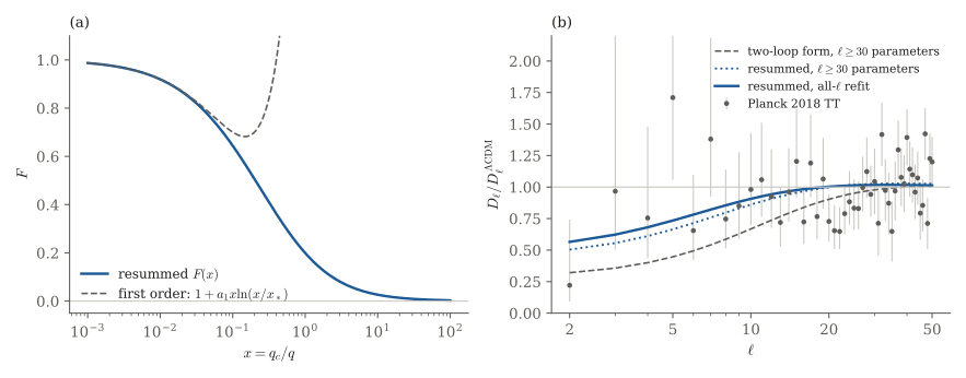
Figure 1. (a) The resummed gauge-field trace correlator (6) and its first-order expansion $1+a_1x\ln(x/x_\ast)$, as functions of $x=q_c/q$. (b) Temperature spectrum relative to the $\Lambda$CDM fit of section 6 at $\ell\le50$, with the Planck 2018 data. The two curves at the published $\ell\ge30$ parameters [ACDGS] have their amplitude matched to $\Lambda$CDM over $30\le\ell\le800$; the solid curve is the $N_B=1$ refit.

Part of the penalty at $\ell\ge30$ comes from fixing the background. Refitting both models on a $3\times3$ grid in $(\omega_b,\omega_c)$, with $\omega_b\in[0.0219,0.0228]$, $\omega_c\in[0.1175,0.1225]$ and the acoustic angle held fixed, and interpolating quadratically, the difference for $N_B=1$ becomes $+4.2$ with a Gaussian prior from the Planck 2018 values $\omega_b=0.02237\pm0.00015$, $\omega_c=0.1200\pm0.0012$ [Planck VI], and $+3.0$ minimised over the grid without a prior; the minimum then lies on the edge $\omega_c=0.1175$. The prior was derived within $\Lambda$CDM from data that include the temperature spectrum, so it favours $\Lambda$CDM slightly. Outside the grid the quadratic interpolation moves both models to $\omega_c\approx0.11$, where the difference nearly vanishes; temperature data to $\ell=800$ do not constrain $\omega_c$ well enough to make that extrapolation meaningful. Over the treatments within the grid, the resummed model is worse than $\Lambda$CDM by $\Delta(-2\ln\mathcal L)=3.0$ to $5.0$ while having one more primordial parameter. As a rough Gaussian equivalent, $\sqrt{\Delta(-2\ln\mathcal L)}$ is $1.7$ to $2.2$.

After the refit, the cost is shared between low and high multipoles: $+2.1$ at $\ell<30$, and $+2.9$ at $\ell\ge30$, mostly from an excess of $1.3$–$1.7\%$ over $\Lambda$CDM at $\ell=30$–$50$. Both are in a regime where the compressed likelihood is adequate in magnitude but not in detail. A fit with the full Planck temperature and polarization likelihood and free background is needed to turn these numbers into a significance.

7. Further consequences

The first two subsections depend on the resummed spectrum (7); the last collects consequences that already follow from the two-loop form (3).

Low-multipole polarization

The suppression of the scalar spectrum at $q\lesssim q_c$ appears in the reionisation bump of the $E$-mode spectrum, which probes the largest scales. At the $N_B=1$ refit and $\tau=0.0544$, $C_\ell^{EE}$ relative to $\Lambda$CDM at $\ell=2,\dots,8$ is $0.45,\ 0.56,\ 0.64,\ 0.69,\ 0.74,\ 0.79,\ 0.85$.

Tensor modes behave differently. The tensor spectrum is inversely proportional to the analogous function $f^T$ of the transverse-traceless part of the correlator, with $f^T_0=N_A/256$ [CDS], and the gauge field is one of the $N_A$ units in $f^T_0$. The crossover changes only that unit, so at leading order the tensor spectrum at low $\ell$ changes by a fraction of at most $1/N_A<1/889\approx1.1\times10^{-3}$. If primordial $B$ modes are detected at low $\ell$, the model predicts an unsuppressed reionisation bump in $BB$ together with a suppressed one in $EE$.

A cosmic-variance-limited measurement of $EE$ at $2\le\ell\le30$ over 70% of the sky, an idealisation of the low-$\ell$ measurement planned by LiteBIRD [LiteBIRD], would separate the two only weakly. With $\tau$ refitted in $\Lambda$CDM at fixed $A_se^{-2\tau}$, the $N_B=1$ spectrum differs from the best $\Lambda$CDM by $\Delta\chi^2=2.0$ (best $\tau=0.051$), and by about $1.5$ using $\ell\le10$ only. Foregrounds and noise would reduce this.

Effective running

A survey that fits $\Lambda$CDM with running, $\ln\Delta^2=\ln A_s+(n_s-1)\ln(q/q_\ast)+\tfrac12\alpha\ln^2(q/q_\ast)$, to data generated by (7) measures an effective running $\alpha_{\rm eff}$, a weighted average of the local running over the scales it probes. At first order in $u$ the local running is $u(L-2)$ with $L=\ln(q/\beta\lvert g\rvert q_\ast)$, since $\ln\Delta^2=\ln\Delta_0^2+uL$ to that order and $d u/d\ln q=-u$, $dL/d\ln q=1$; it changes sign at $L=2$, at $\ell\approx140$ for the $N_B=1$ refit and $\ell\approx180$ for the published $\ell\ge30$ parameters, and is negative at lower $q$. The value of $\alpha_{\rm eff}$ therefore depends on the multipole range and on the weights.

We computed it as the minimum-$\chi^2$ projection of the $TT$, $TE$ and $EE$ spectra of the $N_B=1$ refit onto the template, with Gaussian Fisher metrics and the background fixed. A Planck-like metric has white noise of $33$ and $70\,\mu$K-arcmin in temperature and polarization, a $7'$ beam and $f_{\rm sky}=0.6$ at all multipoles. Over $30\le\ell\le2500$ it gives $\alpha_{\rm eff}=+0.016$; over $2\le\ell\le2500$ it gives about $+0.01$, a value that moves by a few thousandths with the low-$\ell$ sky fraction and noise assumed. A weighting that mimics the Planck and ACT combination of [ACT] uses the Planck-like metric for temperature at $2\le\ell<1000$ and polarization at $2\le\ell<600$, plus an ACT-like survey at $600\le\ell\le3000$ with $15$ and $21\,\mu$K-arcmin, a $1.4'$ beam and $f_{\rm sky}=0.4$; it gives $\alpha_{\rm eff}=+0.011$. The measurement from Planck, ACT, CMB lensing and BAO, $dn_s/d\ln k=0.0062\pm0.0052$ [ACT], lies within about one standard deviation of this. Planck alone gives $-0.0045\pm0.0067$ [Planck X].

These projections hold the background fixed, and marginalising it could shift them. For the $N_B=1$ refit, $\alpha_{\rm eff}$ is positive, of order $+0.01$, in every weighting considered. With the background fixed, a survey with $1\,\mu$K-arcmin noise over 40% of the sky at $30\le\ell\le3000$ would measure $\alpha$ with $\sigma\approx0.0015$; marginalising the background would increase this, by an amount we have not computed.

Consequences of the two-loop form

Write $n_s-1$, $\alpha_s$ and $\beta_s$ for the first three logarithmic derivatives of $\ln\Delta^2$ with respect to $\ln q$ (the tilt, its running and the running of the running).

Proposition 3 (running sum rule). To first order in $u$, the spectrum (3) satisfies

$$n_s-1=-u(L-1),\qquad\alpha_s=u(L-2),\qquad\beta_s=-u(L-3),\qquad L=\ln\frac{q}{\beta\lvert g\rvert q_\ast},$$

and hence

$$\beta_s+2\alpha_s+(n_s-1)=0 \tag{9}$$

at every $q$, for all values of $g$ and $\beta$.

Proof. To first order, $\ln\Delta^2=\ln\Delta_0^2-u\ln(\beta u)=\ln\Delta_0^2+uL$. Write $\partial=d/d\ln q$. Then $\partial u=-u$ and $\partial L=1$, so $(\partial+1)u=0$ and $(\partial+1)(uL)=u$, hence $(\partial+1)^2(uL)=0$. The left side of (9) is $(\partial^3+2\partial^2+\partial)\ln\Delta^2=\partial(\partial+1)^2\ln\Delta^2$, which vanishes because $(\partial+1)^2$ annihilates $uL$ and $\partial$ annihilates the constant. The individual expressions follow by differentiating $uL$ three times.

The resummation does not affect (9) at the pivot, where $x\approx0.004$. With the full forms (3) and (7), the left side of (9) at $q_\ast$ is at most $7\times10^{-4}$ in magnitude for all the parameter sets considered here, while the individual terms are of order $10^{-2}$. At the pivot, (7) at the $N_B=1$ refit gives $n_s=0.975$, $\alpha_s=+0.016$ and $\beta_s=-0.008$; at the published $\ell\ge30$ parameters it gives $0.968$, $+0.020$ and $-0.008$. For these two sets $L=3.3$ and $3.6$ at the pivot, so the leading-order ratio $\alpha_s/(n_s-1)=-(L-2)/(L-1)$ is $-0.57$ to $-0.61$; the full forms give $-0.63$ and $-0.65$. The value $-1$ quoted in [AGS] is its limit for $L\to\infty$. A measurement of $(n_s,\alpha_s,\beta_s)$ tests (9) for any parameters, but current errors on $\beta_s$, of order $0.01$, are too large for this.

The tensor spectrum has the two-loop form (3) with its own parameters, $g_T$ and $\beta_T$, and with $g_T/g$ between $-2/N_A$ and $-8/N_A$ (from eq. 7.10 of [CDS]), so $0<g_T<1.2\times10^{-4}$ for the fitted values of $g$. The tensor tilt at first order is $n_T=w_T(L_T-1)$ with $w_T=g_Tq_\ast/q$ and $L_T=\ln(q/\beta_Tg_Tq_\ast)$. At the pivot, $L_T$ depends on the finite part of the curvature counterterm through the renormalisation scale $\mu_R$ of [CDS] (their eq. 7.11): $L_T=c_T+\ln(q_\ast/\mu_R)$ with $c_T$ between $-2.3$ and $-2.1$. For $\mu_R=q_\ast$, the scheme of [ACDGS], the tilt is red and of order $-10^{-4}$; for $\mu_R<e^{-3.2}q_\ast$ it is blue. The scalar fit does not fix $\mu_R$ when scalars are present, because the scalar $f_2$ contains an infrared-regulated term absent from $f_2^T$. The model therefore does not predict the sign of the tensor tilt.

As $q\to\infty$, $u\to0$ and $\Delta^2\to\Delta_0^2$: the spectrum becomes scale invariant, whereas the red tilt of $\Lambda$CDM continues. At the $N_B=1$ refit the ratio to the $\Lambda$CDM fit is $1.08$ at $q=1\,{\rm Mpc}^{-1}$ and $1.38$ at $10^3\,{\rm Mpc}^{-1}$. With the $k$-space window for $\mu$-type distortions of Chluba, Erickcek and Ben-Dayan [CEB], $\mu\approx2.2\int_{1\,{\rm Mpc}^{-1}}^\infty\Delta^2(q)\,[e^{-\hat q/5400}-e^{-(\hat q/31.6)^2}]\,d\ln q$ with $\hat q=q\,{\rm Mpc}$, the ratio of $\mu$ to its $\Lambda$CDM value is $1.29$–$1.32$ across the parameter sets above. This extrapolates the dual description over eleven e-folds in scale and assumes that the transition out of the non-geometric phase, which requires a change of the dual theory in the ultraviolet [CDS], occurs at $q\gtrsim10^4\,{\rm Mpc}^{-1}$.

8. Limitations and open questions

The low-$\ell$ result rests on (A1)–(A3). For conformally coupled matter it is the leading term of the $1/N_A$ expansion, and the corrections are suppressed by $1/N_A<1.1\times10^{-3}$ by power counting; the counting has not been carried out diagram by diagram to all orders. For $N_B>1$ the mixed diagrams between the scalar trace and the gauge trace are of the same order as the gauge loop and have not been computed, so the spectrum (7) and the bound (8) are then a model. A flavour-singlet quartic coupling would add a second crossover and at least one parameter. The prescription $\mathcal B(0)=0$ rests on Lemma 1, and we add no finite counterterms beyond those of $\int\sqrt\gamma$ and $\int\sqrt\gamma\,R$; a finite curvature-squared term would change the large-$x$ tail $\mathcal F\approx0.27/x$, which is subleading in (7).

The comparison with data uses a compressed temperature likelihood at fixed or gridded background. With it, the resummed model at $N_B=1$ is worse than $\Lambda$CDM by $\Delta(-2\ln\mathcal L)$ between about $3$ and $5$ while having one more primordial parameter. Whether this survives the full Planck likelihood with polarization and a free background, and how the model fares against ACT and SPT data at high $\ell$, has not been determined. The observed quadrupole is $0.39$ times the prediction of the $N_B=1$ refit, against $0.22$ times that of $\Lambda$CDM.

The fitted parameters do not fix a late-time vacuum energy: the only term in the correlator independent of $q$ is the contact term of Lemma 1, which does not enter $\mathcal B$, so a late-time vacuum energy would require ingredients outside the fitted dual theory. The value $b=\tfrac{11}{12}a_1$, if exact, should follow from a closed-form evaluation of (6), which we have not found. It is not known whether a non-perturbative treatment of the dual theory at $\lambda\gtrsim1$, relevant only at $\ell<1$ for the fitted parameters, changes the positivity bound.

References

1. McFadden, Skenderis, “Holography for cosmology,” arXiv:0907.5542.
2. McFadden, Skenderis, “The holographic universe,” arXiv:1001.2007.
3. Afshordi, Corianò, Delle Rose, Gould, Skenderis, “From Planck data to Planck era: observational tests of holographic cosmology,” arXiv:1607.04878.
4. Afshordi, Gould, Skenderis, “Constraining holographic cosmology using Planck data,” arXiv:1703.05385.
5. Corianò, Delle Rose, Skenderis, “Two-point function of the energy-momentum tensor and generalised conformal structure,” arXiv:2008.05346.
6. Giombi, Tarnopolsky, Klebanov, “On $C_J$ and $C_T$ in conformal QED,” arXiv:1602.01076.
7. BICEP/Keck Collaboration, “BICEP/Keck XIII: improved constraints on primordial gravitational waves using Planck, WMAP, and BICEP/Keck observations through the 2018 observing season,” arXiv:2110.00483.
8. Planck Collaboration, “Planck 2018 results. V. CMB power spectra and likelihoods,” arXiv:1907.12875.
9. Planck Collaboration, “Planck 2018 results. VI. Cosmological parameters,” arXiv:1807.06209.
10. Planck Collaboration, “Planck 2018 results. X. Constraints on inflation,” arXiv:1807.06211.
11. Calabrese et al. (ACT Collaboration), “The Atacama Cosmology Telescope: DR6 constraints on extended cosmological models,” arXiv:2503.14454.
12. LiteBIRD Collaboration, “Probing cosmic inflation with the LiteBIRD cosmic microwave background polarization survey,” arXiv:2202.02773.
13. Chluba, Erickcek, Ben-Dayan, “Probing the inflaton: small-scale power spectrum constraints from measurements of the CMB energy spectrum,” arXiv:1203.2681.