Understanding why Large Language Models (LLMs) sometimes ‘hallucinate’—generating fluent but factually incorrect or nonsensical information—is an important challenge. While a complete picture remains elusive, we can construct theoretical models to gain insights. These models allow us to explore how the propensity for hallucination might scale with factors like the volume of training data, the inherent complexity of language, and the way we ask models to generate text. This post delves into one such mathematical exploration. We’ll derive, from a set of foundational assumptions, a lower bound on hallucination probability and examine how this bound is governed by these critical parameters.

Core Concepts and Notation

We begin by defining the essential components and notation used throughout this derivation.

An LLM with parameters $\theta$ models a conditional probability distribution $P(Y \mid X, \theta)$, where $X = (x_1, \ldots, x_{L_X-1})$ is the input context of length $L_X$, and $Y$ is the next token. The model outputs logits $\mathbf{l}(X, \theta) = (l_1, \ldots, l_{N_V})$, where $l_i$ is the logit for the $i$-th token in a vocabulary $V$ of size $N_V$.

The probability of generating a specific token $y_i$ given context $X$ is given by the softmax function applied to the logits:

$$P(y_i \mid X, \theta) = \frac{\exp(l_i)}{\sum_{j=1}^{N_V} \exp(l_j)}$$

When generating text with a temperature parameter $T > 0$, this probability is adjusted:

$$P_T(y_i \mid X, \theta) = \frac{\exp(l_i/T)}{\sum_{j=1}^{N_V} \exp(l_j/T)}$$

A lower temperature ($T \to 0$) makes the distribution sharper (more deterministic), while a higher temperature ($T \to \infty$) makes it flatter (more random).

For a given context $X$, let $y^*(X)$ denote the “correct” or desired next token (e.g., in factual recall tasks where the answer is unambiguous). The hallucination probability is then the probability of not generating this correct token:

$$P_{h}(X, \theta, T) = 1 - P_T(y^*(X) \mid X, \theta)$$

Our goal is to understand how $\bar{P}_{h}$, the average hallucination probability over all contexts, behaves.

Modeling Logits from Corpus Evidence

Our first step is to model how an LLM might arrive at its logits based on its training data. One way to approach this is by considering the behavior of very wide neural networks, a regime often studied through the Neural Tangent Kernel (NTK). In the NTK limit, particularly for networks trained with gradient descent, the output of the network (e.g., a logit for a specific token) can be approximated as a linear function of the initial parameters.

Equivalently, this can be viewed as a sum over contributions from the training data, weighted by the NTK. Specifically, the logit $l_i(X, \theta)$ for a token $y_i$ given a context $X$, after training on a corpus $\mathcal{D} = \{(X_j, y_{\text{target},j})\}_{j=1}^{\vert\mathcal{D}\vert}$, can be expressed in a form like:

$$l_i(X, \theta) \approx \sum_{(X_j, y_{\text{target},j}) \in \mathcal{D}} \alpha_{ij}(X_j, y_{\text{target},j}) \Theta(X, X_j; \theta_0) + b_i$$

Here, $\Theta(X, X_j; \theta_0)$ is the Neural Tangent Kernel evaluated between the current context $X$ and a training context $X_j$ (computed with network parameters at initialization $\theta_0$). The terms $\alpha_{ij}$ are learned coefficients that depend on the specific training example (including the target token $y_{\text{target},j}$ and its relation to $y_i$), and $b_i$ is a bias term.

This formulation suggests that logits are built by accumulating “support” from similar training instances.

For simplicity and tractability in our analysis, we adopt a simplified model inspired by this NTK perspective. We propose that the logit $l_i(X, \theta)$ for a token $y_i$ given context $X$ is primarily determined by how much “support” in the corpus $\mathcal{D}$ favors $y_i$ in this context, versus the total support for any token. The logit is approximated as:

$$l_i(X, \theta) \approx \beta_S E(y_i \mid X) - \beta_C \mathcal{E}_X + c$$

In this model:

• $E(y_i \mid X)$ represents the accumulated support for token $y_i$ in the context $X$, which we can also refer to as its “evidence density”. It is calculated by summing a semantic similarity kernel, $K(X, X_j)$, over all training instances $(X_j, y_{\text{target}})$ from the corpus $\mathcal{D}$ where the target token $y_{\text{target}}$ was indeed $y_i$. The kernel $K(X, X_j)$ measures the relevance of a training context $X_j$ to the current context $X$, with $0 \le K(X,X_j) \le 1$. Formally:

  $$E(y_i \mid X) = \sum_{(X_j, y_{\text{target}}) \in \mathcal{D} \text{ s.t. } y_{\text{target}} = y_i} K(X, X_j)$$

  Intuitively, the more ‘support’ (high-similarity training examples) the model has seen for $y_i$ following a context like $X$, the higher its evidence density $E(y_i \mid X)$ will be. This quantity is bounded by $0 \le E(y_i \mid X) \le N_{y_i}(\mathcal{D})$, where $N_{y_i}(\mathcal{D})$ is the total count of token $y_i$ in the training corpus.

• $\mathcal{E}_X$ represents the total support for any token in the context $X$. It is the sum of the individual evidence densities $E(y_k \mid X)$ for all possible tokens $y_k$ in the vocabulary $V$:

  $$\mathcal{E}_X = \sum_{k=1}^{N_V} E(y_k \mid X)$$

  This can also be expressed as a sum of kernel similarities over all training examples whose contexts $X_j$ are relevant to the current context $X$, regardless of the target token: $\mathcal{E}_X = \sum_{(X_j, y_{\text{target}}) \in \mathcal{D}} K(X, X_j)$. Consequently, $0 \le \mathcal{E}_X \le \vert\mathcal{D}\vert$, the total size of the training corpus.

• $\beta_S > 0$ and $\beta_C \ge 0$ are parameters that scale the influence of these respective support terms, and $c$ is a constant bias term.

This simplified model captures a competitive dynamic: a token $y_i$ gains logit strength proportional to its specific support $E(y_i \mid X)$, but this is counteracted by the total support $\mathcal{E}_X$ for all tokens in that context. Essentially, a token’s logit is determined by its own support, penalized by a measure of the ‘background’ support for all tokens in that context. This form, while simplified, allows for a more tractable analysis of hallucination probability.

Condition for Bounded Hallucination

Now, let’s consider what it takes for the hallucination probability $P_{h}(X, \theta, T)$ for a specific context $X$ to be below a chosen threshold $\epsilon_0 \in (0,1)$. If $P_{h}(X, \theta, T) \le \epsilon_0$, then the probability of generating the correct token $y^*(X)$ must be $P_T(y^*(X) \mid X, \theta) \ge 1 - \epsilon_0$.

This implies that the logit of the correct token $l_{y^*}$ must be sufficiently larger than the logit of any other token $l_{y_{\text{alt}}}$. For the highest-logit alternative token $y_{\text{alt}}$, and assuming a large vocabulary $N_V$, this condition can be shown to require:

$$l_{y^*}(X, \theta) - l_{y_{\text{alt}}}(X, \theta) \ge T \log\left(\frac{1 - \epsilon_0}{\epsilon_0}\right)$$

Substituting our simplified logit model into this inequality, we get a condition on the difference in evidence densities:

$$E(y^*(X) \mid X) - E(y_{\text{alt}} \mid X) \ge \frac{T \log\left(\frac{1 - \epsilon_0}{\epsilon_0}\right)}{\beta_S}$$

Let’s define the right-hand side as $M'(\epsilon_0, T) = \frac{T \log\left(\frac{1 - \epsilon_0}{\epsilon_0}\right)}{\beta_S}$. This term $M'$ represents the minimum evidence advantage the correct token must have over its strongest competitor. If $E(y^*(X) \mid X) - E(y_{\text{alt}} \mid X) < M'(\epsilon_0, T)$, then $P_{h}(X, \theta, T) > \epsilon_0$.

In simpler terms, for the model to avoid hallucinating (with probability at least $1-\epsilon_0$) in a given instance, the ‘evidence signal’ for the correct token $y^*$ must exceed the evidence for the strongest competitor $y_{\text{alt}}$ by this margin $M'$. This margin depends on our desired confidence (related to $\epsilon_0$) and the generation temperature $T$. A higher temperature or a stricter (smaller) $\epsilon_0$ demands a larger evidence gap.

Aggregate Hallucination and Data Sparsity

Deriving the exact average hallucination probability $\bar{P}_{h}$ is complex. Instead, we seek a lower bound. To make progress, we consider a simplified (and stronger) condition for when $P_{h}(X, \theta, T) > \epsilon_0$: we assume this happens if the total evidence density for the context, $\mathcal{E}_X$, is less than the required evidence margin $M'(\epsilon_0, T)$.

The intuition is that if the overall evidence available for any token in a given context $X$ is very low (i.e., the context is highly unfamiliar or ambiguous based on the training data, such that $\mathcal{E}_X < M'$), it becomes difficult for the correct token $y^*$ to gather enough evidence to significantly surpass alternatives by the necessary margin. This simplification allows us to use aggregate statistics of $\mathcal{E}_X$ to derive a bound.

1. Average Total Evidence: The average total evidence density, $\bar{\mathcal{E}}_X$, taken over all possible contexts $X$ (assuming a uniform distribution over a context space of size $N_V^{L_X-1}$), is:

$$\bar{\mathcal{E}}_X = \mathbb{E}_{X}[\mathcal{E}_X] = \frac{\vert\mathcal{D}\vert \bar{S}}{N_V^{L_X-1}}$$

Where:

• $\vert\mathcal{D}\vert$ is the size of the training corpus.
• $\bar{S}$ is the average kernel influence (effectively, how many contexts $X$ are ‘covered’ by an average training example $X_j$).
• $N_V^{L_X-1}$ approximates the size of the unique context space. This shows that average evidence density increases with corpus size and decreases with the vastness of the language space.

2. Lower Bound on Fraction of Low-Evidence Contexts: Let $f(\epsilon_0)$ be the fraction of contexts for which $\mathcal{E}_X < M'(\epsilon_0, T)$. For these contexts, by our simplifying assumption, $P_{h}(X, \theta, T) > \epsilon_0$. Using Markov’s inequality, which states $P(Z \ge a) \le \mathbb{E}[Z]/a$ for a non-negative random variable $Z$, we have $P(\mathcal{E}_X \ge M'(\epsilon_0, T)) \le \frac{\bar{\mathcal{E}}_X}{M'(\epsilon_0, T)}$. Therefore, the fraction of low-evidence contexts is bounded:

$$f(\epsilon_0) = P(\mathcal{E}_X < M'(\epsilon_0, T)) \ge 1 - \frac{\bar{\mathcal{E}}_X}{M'(\epsilon_0, T)}$$

This bound is informative (i.e., $f(\epsilon_0) > 0$) if $\bar{\mathcal{E}}_X < M'(\epsilon_0, T)$.

Let $L(\epsilon_0) = \log\left(\frac{1 - \epsilon_0}{\epsilon_0}\right)$. This term increases as $\epsilon_0$ gets closer to 0 or 1, reflecting a demand for a larger logit gap. Let $C = \bar{S} \beta_S$ be a constant that groups model structure and kernel properties. The ratio then becomes $\frac{\bar{\mathcal{E}}_X}{M'(\epsilon_0, T)} = \frac{C \vert\mathcal{D}\vert}{N_V^{L_X-1} T L(\epsilon_0)}$. So, the lower bound on $f(\epsilon_0)$ is:

$$f(\epsilon_0) \ge 1 - \frac{C \vert\mathcal{D}\vert}{N_V^{L_X-1} T L(\epsilon_0)}$$

3. Lower Bound on Average Hallucination: The average hallucination probability $\bar{P}_{h} = \mathbb{E}_{X} [P_{h}(X, \theta, T)]$ can be lower-bounded because, for the fraction $f(\epsilon_0)$ of contexts, $P_{h} > \epsilon_0$ and thus $\bar{P}_{h} > \epsilon_0 \cdot f(\epsilon_0)$.

Substituting the bound for $f(\epsilon_0)$ gives

$$\bar{P}_{h} > \epsilon_0 \left(1 - \frac{C \vert\mathcal{D}\vert}{N_V^{L_X-1} T L(\epsilon_0)}\right)$$

This inequality is a lower bound on the average hallucination probability. Let’s break down the term $k_0(\epsilon_0) = \frac{C \vert\mathcal{D}\vert}{N_V^{L_X-1} T L(\epsilon_0)}$:

• $C \vert\mathcal{D}\vert$ represents the ‘total effective evidence’ in the corpus, scaled by model and kernel parameters.
• $N_V^{L_X-1}$ is the vastness of the potential context space.
• $T L(\epsilon_0)$ represents the ‘difficulty’ of distinguishing the correct token, influenced by temperature and our chosen hallucination threshold $\epsilon_0$.

If this ratio $k_0(\epsilon_0)$ (representing data richness relative to task difficulty for a given $\epsilon_0$) is small (i.e., $k_0(\epsilon_0) \ll 1$), the term in the parenthesis approaches 1, and the bound approaches $\epsilon_0$. If $k_0(\epsilon_0)$ is large, the bound can become smaller. This expression already hints at the scaling relationships we’re looking for, but it still depends on our arbitrary choice of $\epsilon_0$.

Optimizing the Lower Bound

The derived lower bound $g(\epsilon_0) = \epsilon_0 (1 - k_0(\epsilon_0))$ depends on our choice of $\epsilon_0$. We can find the tightest possible bound by choosing $\epsilon_0$ to maximize $g(\epsilon_0)$. Let $k = \frac{C \vert\mathcal{D}\vert}{N_V^{L_X-1} T}$ be the key scaling parameter, which encapsulates data density ($\vert\mathcal{D}\vert/N_V^{L_X-1}$), model characteristics ($C$), and inverse temperature ($1/T$). The bound is $g(\epsilon_0) = \epsilon_0 (1 - \frac{k}{L(\epsilon_0)})$.

The optimal $L^* = L(\epsilon_0^*)$ that maximizes $g(\epsilon_0)$ (where $\epsilon_0^*$ is the optimal threshold) is found by solving the following transcendental equation:

$$(L^*)^2 = k \left(L^* + 1 + e^{-L^*}\right)$$

While this equation doesn’t have a simple closed-form solution for $L^*$, its properties can be analyzed, especially in asymptotic regimes (when $k$ is very small or very large). This $L^*$ represents an optimal ‘logit difference scale’ that balances making $\epsilon_0^*$ small (desirable for the $\epsilon_0^*$ factor in the bound) versus making the term $(1 - k/L^*)$ large.

The optimized value $\epsilon_0^*$ is then $\frac{1}{1+e^{L^*}}$. Substituting $\epsilon_0^*$ and $L^*$ into $g(\epsilon_0)$ gives the optimized lower bound on average hallucination:

$$\bar{P}_{h} > \frac{1}{1+e^{L^*}} \left(1 - \frac{k}{L^*}\right)$$

This is our main result: a lower bound on average hallucination probability that depends on the consolidated parameter $k$.

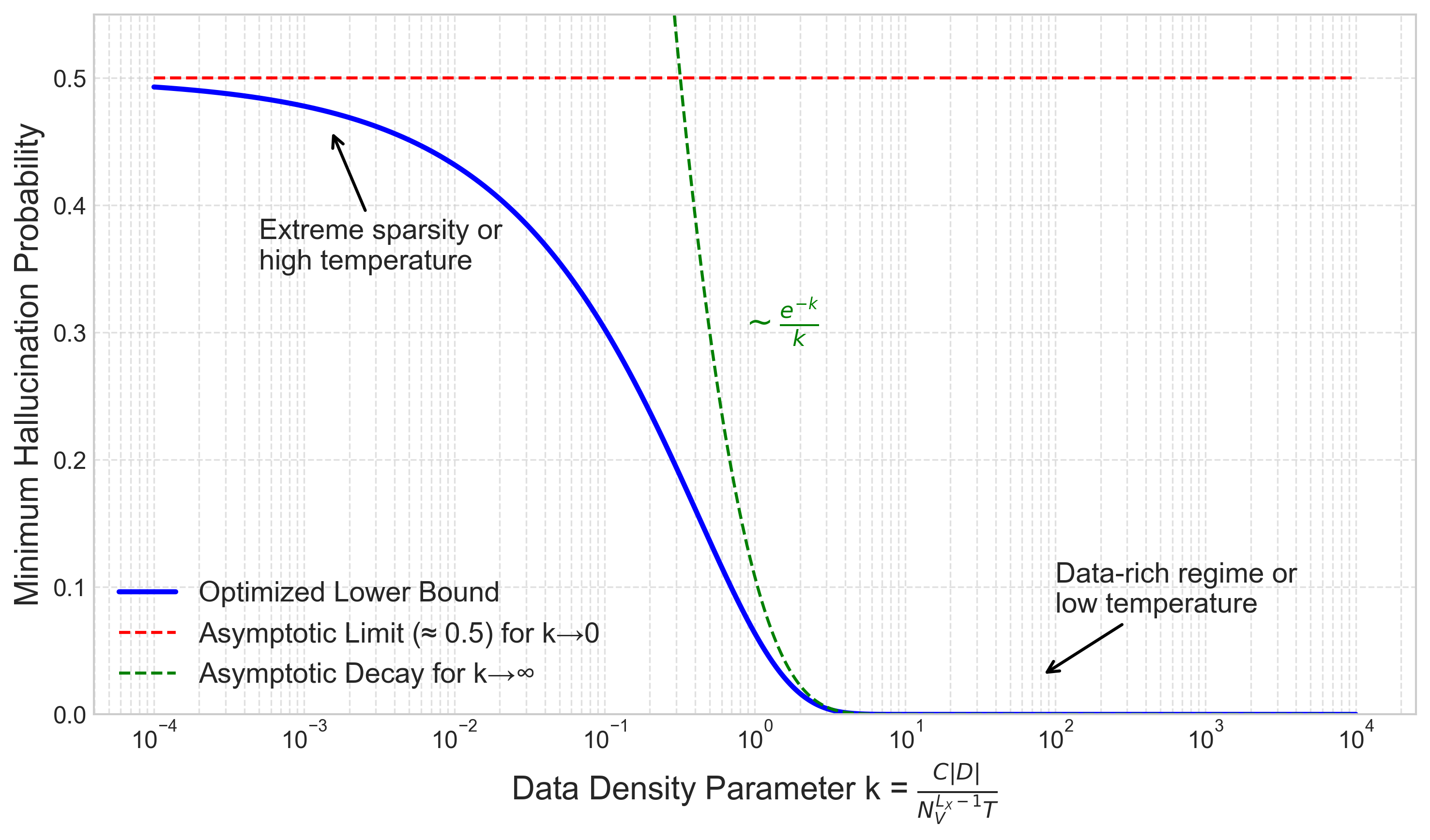Figure 1: The optimized lower bound on average hallucination probability, $\bar{P}_{h}$, as a function of the data density, model, and temperature parameter $k = \frac{C \vert\mathcal{D}\vert}{N_V^{L_X-1} T}$. The bound transitions from $\approx 0.5$ for small $k$ (sparse data/high temperature) towards $0$ for large $k$ (dense data/low temperature).

We can derive the behavior of this optimized bound in limiting cases of the parameter $k$:

1. $k \to 0$ (Extreme Data Sparsity or High Temperature) In this regime, data is very scarce relative to language complexity, or generation is very random. It can be shown that $L^* \approx \sqrt{2k}$, which approaches 0. As $L^* \to 0$, $\epsilon_0^* = \frac{1}{1+e^{L^*}} \to \frac{1}{2}$. Further analysis shows the entire bound $\bar{P}_{h} \to \frac{1}{2}$. This suggests that with very sparse data or at very high temperatures, the model’s output is nearly random concerning correctness, leading to an average hallucination probability of at least 50%. This makes intuitive sense: if the model has very little reliable information from its training ($k \to 0$), its performance should degrade towards random guessing. For a binary decision of ‘correct’ vs ‘any incorrect alternative’, random guessing would yield a 50% error rate.

2. $k \to \infty$ (Data-Rich Regime or Low Temperature) In this regime, data is abundant, or generation is nearly deterministic. It can be shown that $L^* \approx k$. Then $\epsilon_0^* = \frac{1}{1+e^{L^*}} \approx e^{-L^*}$ $\approx e^{-k}$. The term $(1 - k/L^*)$ approaches 0. More precisely, the bound $\bar{P}_{h}$ decays towards 0, approximately as $\frac{e^{-k}}{k}$. This indicates that with sufficiently dense data and low temperature, the derived lower bound on hallucination can be made arbitrarily small, decaying exponentially with $k$. This is also intuitive: if we have abundant data relative to complexity and low randomness ($k \to \infty$), the model should be able to learn the correct patterns effectively, and the floor for hallucination should drop significantly.

Conclusion

This derivation provides a theoretical lower bound on the average hallucination probability in LLMs, starting from a model of how corpus evidence translates to logits. It formally demonstrates how this hallucination floor scales with fundamental parameters, encapsulated in the parameter $k = \frac{C \vert\mathcal{D}\vert}{N_V^{L_X-1} T}$:

• Corpus Size ($\vert\mathcal{D}\vert$): Larger datasets tend to decrease the bound (increase $k$).
• Context Space Complexity ($N_V^{L_X-1}$): Larger vocabularies or longer contexts increase complexity and tend to increase the bound (decrease $k$).
• Generation Temperature ($T$): Higher temperatures tend to increase the bound (decrease $k$).
• Model/Kernel Properties ($C$): Factors like effective semantic similarity spread also play a role.

It is important to remember that this model, while illustrative, is a significant simplification of the complex mechanisms underlying LLM behavior, and does not encompass more intricate forms of hallucination. Note that the exact form of the scaling we derived here is predicated on the softmax function. A natural follow-up question is whether there is an alternative to softmax that would result in qualitatively better scaling behavior.