Quantum Gravity

A proof of the coth joint conjecture for regions between two spacelike or null polygonal curves

The Benincasa–Dowker action is a proposed action for causal sets. For a causal set sprinkled at density $\rho$ into a region of Minkowski space its mean is expected to approach, as $\rho\to\infty$, the Einstein–Hilbert action plus a term carried by the joints, the codimension-two surfaces where the past and future boundaries of the region meet. Dowker, Liu and Lloyd-Jones conjectured that a joint at which the two boundaries meet at Lorentzian angle $\theta$ contributes $\coth\theta$ per unit joint area in Planck units. We prove this for flat two-dimensional regions bounded by two polygonal spacelike or null curves, and for the products of such regions with a flat plane in four dimensions.

In two dimensions the regions are those bounded below and above by piecewise-linear spacelike or null curves that meet only at their two endpoints, convex or not. For them the mean action tends to $\coth\theta_L+\coth\theta_R$, the sum over the two joints, with error $O(\rho^{-1})$. In four dimensions, for the product of such a region with a flat transverse plane, the mean action is proportional to the transverse area $A$ and tends to $(A/\ell_p^2)(\coth\theta_L+\coth\theta_R)$ with relative error $O(\rho^{-1/2})$. In particular no logarithm of $\rho$ appears and the flat spacelike faces contribute nothing. Joints along which $\theta$ varies, curved faces, non-product regions in four dimensions and timelike boundaries are not covered.

The same expansion gives a result in curved space. For the two-dimensional metric $(1+2\phi)\eta$, at first order in $\phi$, every causal interval has mean action $2+\tfrac12\int R\sqrt{-g}\,d^2x$ up to an error of order $\phi\,\rho^{-1}\log\rho$, terms of order $\phi^2$ and terms exponentially small in $\rho$ times the interval volume, whatever the profile of the curvature inside the interval.

The action was introduced by Benincasa and Dowker [BD]. For a causal interval in flat space, Buck, Dowker, Jubb and Surya [BDJS] found the mean exactly in two dimensions, $2(1-e^{-\rho V})$, and showed for $d=2,\dots,16$ that it tends to the volume of the joint in Planck units. Dowker [D20] and Machet and Wang [MW] found the Einstein–Hilbert term plus the joint volume for causal intervals in weakly curved spacetimes, at first order in a curvature that is constant over the interval to the order considered. Dowker, Liu and Lloyd-Jones [DLLJ] found that a joint between two spacelike boundaries contributes more than its volume and conjectured the weight $\coth\theta$ (their Conjecture 1′, eqs. 11 and 68, stated also for curved joints along which $\theta$ varies). They computed the mean by integrating over the separation vector of a pair of points, weighted by the “volume of realisation”, the volume of the overlap of the region with its translate by minus that vector; they attribute this method to an MSc dissertation of Chevalier (their ref. 25). With it they supported the conjecture with the two-dimensional lozenge and spacelike triangle, evaluated with an enlarged integration region valid at large $\rho$, and with $d$-dimensional cones of constant $\theta$, checked up to $d=11$. The overlap function $K$ used below is twice their volume of realisation, the factor coming from null coordinates. Our contribution is an exact proof for the classes above, in which the two joints may have different angles, with each joint’s contribution obtained as a second derivative of $K$ at zero separation (Lemma 2) and with error bounds that exclude logarithmic and face terms. The curved result extends [D20] and [MW] from approximately constant curvature to an arbitrary profile, at linear order.

The reader is assumed to know what a causal set and a Poisson sprinkling are. Signature is mostly plus, and the Lorentzian angle between two spacelike directions of rapidities $\eta_1,\eta_2$ is $\lvert\eta_1-\eta_2\rvert$.

1. The mean action

Sprinkle a region $M$ of a spacetime with a Poisson process of density $\rho$ and give the points the causal order. For $k\ge0$ let $N_k$ be the number of related pairs $p\prec q$ with exactly $k$ sprinkled points strictly between them, so that $N_0$ counts links, and let $N$ be the number of points. The two- and four-dimensional actions are [DLLJ]

$$S_2=2\,(N-2N_0+4N_1-2N_2),\qquad S_4=\frac{4}{\sqrt6}\Big(\frac{\ell}{\ell_p}\Big)^2\big(N-N_0+9N_1-16N_2+8N_3\big),$$

where $\ell=\rho^{-1/4}$ is the discreteness length and $\ell_p^2=8\pi G_{\rm N}$. (Our $N_k$ is their $N_{k+1}$.) Let $V_{pq}$ be the volume of the causal interval between $p\prec q$. If $M$ is causally convex, which holds for every region in this note, the number of points inside that interval is Poisson with mean $\rho V_{pq}$, so $\langle N_k\rangle=\rho^2\iint_{p\prec q}dV_p\,dV_q\,(\rho V_{pq})^ke^{-\rho V_{pq}}/k!$, and the mean action is

$$\langle S_d\rangle=c_d\Big[\rho V_M+\rho^2\!\int_M\!dV_p\!\int_{M\cap J^+(p)}\!dV_q\;F_d(\rho V_{pq})\Big], \tag{1}$$

with $c_2=2$, $c_4=(4/\sqrt6)(\ell/\ell_p)^2$, and kernels whose coefficients are those of $S_d$ divided by $k!$:

$$F_2(\lambda)=(-2+4\lambda-\lambda^2)\,e^{-\lambda},\qquad F_4(\lambda)=\big(-1+9\lambda-8\lambda^2+\tfrac43\lambda^3\big)\,e^{-\lambda}.$$

Both terms in the bracket grow with $\rho$, and the finite limit comes from cancellations between them. Their bookkeeping is done by the Mellin transforms of the kernels,

$$\int_0^\infty\lambda^{s-1}F_d(\lambda)\,d\lambda=\Gamma(s)\,Q_d(s),\qquad Q_2(s)=-(s-1)(s-2),\quad Q_4(s)=\tfrac13(2s-1)(s-1)(2s-3), \tag{2}$$

which follow from $\int_0^\infty\lambda^{s+k-1}e^{-\lambda}d\lambda=\Gamma(s)\,(s)_k$. We use only the values

$$Q_2'(1)=1,\quad Q_2'(2)=-1,\qquad Q_4(\tfrac12)=Q_4(1)=Q_4(\tfrac32)=0,\quad Q_4'(1)=-\tfrac13,\quad Q_4'(\tfrac32)=\tfrac23 .$$

Roughly, each term $\rho^{k}$ in the bracket of (1) comes with a factor $Q_d$ evaluated at a definite point. Where that point is a zero of $Q_d$ the term drops out, unless the integrand also carries a logarithm, in which case $Q_d'$ survives. The joint terms are of this second kind. They come from logarithms produced by pairs of points that are close in both null directions at once, and the zero of $Q_d$ at the joint exponent ($s=2$ in two dimensions, $s=\tfrac32$ in four) removes the accompanying $\log\rho$ and leaves a finite coefficient. Section 2 reduces (1) to a one-variable integral, section 3 carries out the bookkeeping, and section 4 computes the coefficient.

2. Reduction to one variable

In two dimensions use coordinates $(t,x)$ and null coordinates $u=t-x$, $w=t+x$, so that $dt\,dx=\tfrac12du\,dw$. Two points are related, $p\prec q$, exactly when $q-p=(a,b)$ in null components with $a,b\ge0$, and then $V_{pq}=ab/2$. For a region $P$ in the plane define

$$K(a,b)=\int du\,dw\;\mathbf 1_P(z)\,\mathbf 1_P\big(z+(a,b)\big),$$

the $du\,dw$-area of the set of points $z\in P$ whose translate by $(a,b)$ is still in $P$. Since $V_{pq}$ depends only on $q-p$, the pair integral in (1) is $\tfrac14\rho^2\int_{a,b>0}K(a,b)\,F_2(\rho ab/2)\,da\,db$. Grouping the separations by the product $\mu=ab$ gives

$$\rho^2\!\iint_{p\prec q}\!dV_pdV_q\,F_2(\rho V_{pq})=\frac{\rho^2}{4}\int_0^\infty H(\mu)\,F_2(\rho\mu/2)\,d\mu,\qquad H(\mu)=\int_0^\infty K\Big(a,\frac{\mu}{a}\Big)\frac{da}{a}. \tag{3}$$

The function $H$ is the density of pairs whose causal interval has volume $\mu/2$.

In four dimensions take $M=P\times T^2$, where $T^2$ is a flat torus of area $A$ in the transverse coordinates $x_\perp$, large enough that no causal interval of $M$ wraps around it. (Equivalently, work per unit transverse area of $P\times\mathbb R^2$.) For two points with null separation $(a,b)$ in $P$ and transverse separation $\Delta$ the proper time $\tau$ satisfies $\tau^2=ab-\lvert\Delta\rvert^2$, and the interval volume is $V=\tfrac{\pi}{24}\tau^4$. The transverse integral can be done exactly: with $Y=ab-\lvert\Delta\rvert^2$,

$$\int_{\lvert\Delta\rvert^2<ab}d^2\Delta\;F_4\Big(\frac{\pi\rho}{24}(ab-\lvert\Delta\rvert^2)^2\Big)=\pi\int_0^{ab}F_4\Big(\frac{\pi\rho}{24}Y^2\Big)dY .$$

Write $\sigma=(24/\pi\rho)^{1/2}$ and $\Psi(t)=\int_0^tF_4(y^2)\,dy$. The right-hand side is $\pi\sigma\,\Psi(ab/\sigma)$, and inserting it into (1), with $d^4x=\tfrac12du\,dw\,d^2x_\perp$, gives the pair integral per unit transverse area as $\tfrac{\rho^2}{4}\pi\sigma\int_0^\infty H(\mu)\Psi(\mu/\sigma)\,d\mu$, that is,

$$\frac{1}{A}\,\rho^2\!\iint_{p\prec q}\!dV_pdV_q\,F_4(\rho V_{pq})=6\rho\int_0^\infty\Psi(t)\,H(\sigma t)\,dt, \tag{4}$$

with the same $H$ as in (3). The four-dimensional problem for $P\times T^2$ is therefore the two-dimensional one with a different kernel. The kernel $\Psi$ decays like a Gaussian, because $\Psi(\infty)=\tfrac12\Gamma(\tfrac12)Q_4(\tfrac12)=0$ by (2).

3. The large-density expansion

Everything now depends on the behaviour of $H(\mu)$ as $\mu\to0$, that is, on pairs whose interval is small. The following lemma turns a small-$\mu$ expansion of $H$ into a large-$\rho$ expansion of the action, using nothing but the moments (2).

Lemma 1 (moments). Let $f$ be a continuous function on $(0,\infty)$ bounded by a polynomial times $e^{-\lambda}$, and let $m(s)=\int_0^\infty\lambda^{s-1}f(\lambda)\,d\lambda$. Let $H$ be integrable on $(0,\infty)$ and satisfy, for all $\mu>0$,

$$H(\mu)=\sum_{k=0}^{n_0}\mu^k\big(\alpha_k\log\tfrac1\mu+\beta_k\big)+R(\mu).$$

If $\lvert R(\mu)\rvert\le C\mu^{n_0+1}$, then, as $Z\to\infty$,

$$\int_0^\infty H(\mu)f(Z\mu)\,d\mu=\sum_{k=0}^{n_0}Z^{-k-1}\Big[\alpha_k\big(m(k+1)\log Z-m'(k+1)\big)+\beta_k\,m(k+1)\Big]+O\big(Z^{-n_0-2}\big).$$

If instead $\lvert R(\mu)\rvert\le C\mu^{n_0+1}(1+\lvert\log\mu\rvert)$, the same holds with remainder $O(Z^{-n_0-2}\log Z)$. Both statements hold also for $f=\Psi$, whose Mellin transform is $m_\Psi(s)=-\tfrac{1}{2s}\Gamma\big(\tfrac{s+1}{2}\big)Q_4\big(\tfrac{s+1}{2}\big)$.

Proof. Substitute $\mu=\lambda/Z$. A term $\mu^k\log(1/\mu)$ gives $Z^{-k-1}\int_0^\infty\lambda^k(\log Z-\log\lambda)f(\lambda)\,d\lambda=Z^{-k-1}\big(m(k+1)\log Z-m'(k+1)\big)$, and $\mu^k$ gives $Z^{-k-1}m(k+1)$. The remainder is bounded by $CZ^{-n_0-2}\int_0^\infty\lambda^{n_0+1}\lvert f(\lambda)\rvert\,d\lambda$ in the first case and by $CZ^{-n_0-2}\int_0^\infty\lambda^{n_0+1}(1+\lvert\log\lambda\rvert+\log Z)\lvert f(\lambda)\rvert\,d\lambda$ in the second. For $\Psi$, which is bounded by a polynomial times $e^{-t^2}$, integrate by parts: $\int_0^\infty t^{s-1}\Psi(t)\,dt=-\tfrac1s\int_0^\infty t^sF_4(t^2)\,dt=-\tfrac1{2s}\Gamma\big(\tfrac{s+1}2\big)Q_4\big(\tfrac{s+1}2\big)$, the boundary terms vanishing because $\Psi(0)=\Psi(\infty)=0$.

The bound on $R$ is required for all $\mu$, not only for small $\mu$. In the applications below this follows from the small-$\mu$ bound, because there $H$ is bounded on $[\mu_1,\infty)$ for every $\mu_1>0$ and vanishes for large $\mu$, while the sum grows only like $\mu^{n_0}\log\mu$. The distinction between the two remainders matters: a term $\mu^2\log(1/\mu)$ in $H$ would contribute $Z^{-3}m_{F_2}(3)\log Z$ with $m_{F_2}(3)=-4$, or $Z^{-3}m_\Psi(3)\log Z$ with $m_\Psi(3)=-\tfrac16$, so a logarithm-free remainder in $H$ is what excludes a logarithm at the next order in $\rho$.

We apply the lemma with $n_0=1$ and the logarithm-free remainder to the two-dimensional pair integral (3), with $f=F_2$ and $Z=\rho/2$. By (2), $m(1)=Q_2(1)=0$, $m(2)=Q_2(2)=0$, $m'(1)=Q_2'(1)=1$ and $m'(2)=Q_2'(2)=-1$, so the constants $\beta_0,\beta_1$ and every $\log\rho$ drop out, and

$$\frac{\rho^2}{4}\int_0^\infty H(\mu)F_2(\rho\mu/2)\,d\mu=-\frac{\rho}{2}\alpha_0+\alpha_1+O(\rho^{-1}). \tag{5}$$

For the four-dimensional integral (4) take $f=\Psi$ and $Z=1/\sigma$, so that the left side of (4) is $6\rho\sigma^{-1}\int_0^\infty H(\mu)\Psi(\mu/\sigma)\,d\mu$. Here $m_\Psi(1)=-\tfrac12Q_4(1)=0$, $m_\Psi(2)=-\tfrac14\Gamma(\tfrac32)Q_4(\tfrac32)=0$, $m_\Psi'(1)=-\tfrac14Q_4'(1)=\tfrac1{12}$ and $m_\Psi'(2)=-\tfrac18\Gamma(\tfrac32)Q_4'(\tfrac32)=-\tfrac{\sqrt\pi}{24}$. Hence

$$6\rho\int_0^\infty\Psi(t)H(\sigma t)\,dt=-\frac{\rho}{2}\alpha_0+\frac{\sqrt\pi}{4}\,\rho\,\sigma\,\alpha_1+O(1)=-\frac\rho2\alpha_0+\frac{\sqrt6}{2}\,\rho^{1/2}\alpha_1+O(1). \tag{6}$$

The structure is the same in both dimensions. The constants $\beta_k$, which encode the size and shape of the region, never contribute, because they meet zeros of $Q_d$. The coefficient $\alpha_0$ of $\log(1/\mu)$ produces a term linear in $\rho$. The coefficient $\alpha_1$ of $\mu\log(1/\mu)$ is the only other input to the finite part.

For the regions of this note $\alpha_0=K(0,0)$, which is the $du\,dw$-area of $P$, twice its volume $V_P$. The linear terms in (5) and (6) are then $-\rho V_P$ per unit transverse area, and they cancel the $\rho V_M$ in (1). What remains is

$$\langle S_2\rangle=2\alpha_1+O(\rho^{-1}),\qquad \langle S_4\rangle=\frac{A}{\ell_p^2}\big(2\alpha_1+O(\rho^{-1/2})\big), \tag{7}$$

where in four dimensions we used $c_4\cdot\tfrac{\sqrt6}{2}\rho^{1/2}=2/\ell_p^2$, since $\ell^2\rho^{1/2}=1$. These hold as soon as $H(\mu)=\alpha_0\log\frac1\mu+\beta_0+\mu(\alpha_1\log\frac1\mu+\beta_1)+O(\mu^2)$ with a remainder free of logarithms. It remains to show that $H$ has this form and to compute $\alpha_1$.

4. The overlap function near zero separation

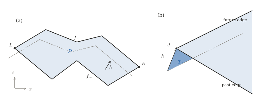
Definition (graph region). A graph region is a set $P=\{(t,x):x_L\le x\le x_R,\ f_-(x)\le t\le f_+(x)\}$ where $f_\pm$ are continuous and piecewise linear with slopes in $[-1,1]$, $f_-<f_+$ on $(x_L,x_R)$ and $f_-=f_+$ at $x_L$ and $x_R$. The graphs of $f_-$ and $f_+$ are the past and future boundaries, and their common endpoints $L$ and $R$ are the joints. At a joint let $v_-\ne v_+$ be the slopes of the past and future edges that end there; the joint angle is $\theta_J=\lvert\operatorname{artanh}v_+-\operatorname{artanh}v_-\rvert\in(0,\infty]$, with $\theta_J=\infty$ if either edge is null, and $\coth\infty=1$.

Every edge is spacelike or null, and the joint angle is the Lorentzian angle of [DLLJ] between the tangents to the past and future boundaries. Every convex polygon with spacelike or null edges is a graph region, with its joints at the leftmost and rightmost vertices; non-convex regions such as the one in figure 1(a) are included too. A graph region is causally convex. Because $f_\pm$ have slopes at most 1 in magnitude and meet at $R$, every point of $P$ satisfies $\lvert t-t_R\rvert\le x_R-x$, so $P$ lies in the left Rindler wedge of $R$; likewise it lies in the right Rindler wedge of $L$. Both wedges are causally convex, so a causal curve between two points of $P$ stays in the strip $x_L\le x\le x_R$, and there $t-f_+(x)$ and $t-f_-(x)$ are non-decreasing along it. Hence it stays in $P$, and (1) applies with full causal diamonds as intervals.

The next lemma rests on a simple picture. The deficit $\lvert P\rvert-K(h)$ is the area of the points of $P$ whose translate by $h$ leaves $P$. For a future-timelike $h$ these points form a strip of width proportional to $h$ under the future boundary, whose area is linear in $h$, except near the two joints, where the strip runs into the past boundary and is cut off. Each cut-off piece is a triangle whose area is quadratic in $h$, and its mixed derivative gives the joint’s contribution.

Lemma 2 (joint triangles). Let $P$ be a graph region and $\lvert P\rvert$ its $du\,dw$-area. At each joint $J$ let $e_-$ and $e_+$ be non-zero vectors along the past and future edges ending at $J$, and write $e\times e'=e^ue'^w-e^we'^u$ for the cross product in null components. There are $\delta_0>0$ and a linear function $\mathcal L(a,b)$ such that, with $h=(a,b)$, for $0\le a,b<\delta_0$

$$K(a,b)=\lvert P\rvert-\mathcal L(a,b)+T_L(a,b)+T_R(a,b),\qquad T_J(a,b)=\frac{\lvert h\times e_+\rvert\,\lvert h\times e_-\rvert}{2\,\lvert e_-\times e_+\rvert}. \tag{8}$$

In particular $\partial_a\partial_bK=\tfrac12(\coth\theta_L+\coth\theta_R)$ on $[0,\delta_0)^2$.

Proof. Fix $h=(a,b)$ with $a,b>0$. In $(t,x)$ components $h_t=\tfrac12(a+b)$ and $h_x=\tfrac12(b-a)$, so $h_t>\lvert h_x\rvert$ and $h$ is future timelike. Along the segment $z+sh$, $s\ge0$, both $t-f_+(x)$ and $t-f_-(x)$ increase strictly, because the slopes of $f_\pm$ are at most 1 in magnitude. Hence, for $z\in P$, the set of $s\ge0$ with $z+sh\in P$ is an interval $[0,s^*(z)]$, and the exit point $z+s^*h$ lies on the future boundary. (If the segment reached $x=x_R$ inside $P$, then $f_-(x_R)\le t\le f_+(x_R)=f_-(x_R)$ there, so it would be at the joint $R$, which is on the future boundary.) The same argument applied to $-h$ shows that, for $y$ on the future boundary, the set of $s\ge0$ with $y-sh\in P$ is an interval $[0,\bar s(y)]$.

Let $E(h)=\{z\in P:z+h\notin P\}$, so that $K(h)=\lvert P\rvert-\lvert E(h)\rvert$. By the above, $z\in E(h)$ exactly when $z=y-sh$ for a point $y=(f_+(x),x)$ of the future boundary and some $s\in[0,1)$ with $s\le\bar s(y)$, and $y,s$ are then unique. In the coordinates $(x,s)$ the area element is $2\big(h_t-f_+'(x)h_x\big)\,dx\,ds$ in $du\,dw$-area, which is positive. Therefore

$$\lvert E(h)\rvert=\int_{x_L}^{x_R}2\big(h_t-f_+'(x)h_x\big)\,dx\;-\;\lvert E'(h)\rvert,\qquad E'(h)=\{y-sh:\ \bar s(y)<s<1\}.$$

The first term is linear in $h$; call it $\mathcal L(h)$. The set $E'(h)$ consists of points $y-sh$ that have crossed the past boundary. The two boundaries are polygonal and meet only at $L$ and $R$, at non-zero angles, so there is a constant $C_P$ such that a point $y$ of the future boundary at distance more than $C_P\lvert h\rvert$ from both joints has $\bar s(y)>1$. Thus $E'(h)$ lies within distance $(C_P+1)\lvert h\rvert$ of the joints. Choose $\delta_0$ so small that within this distance of each joint, $P$ coincides with the wedge bounded by the two edges ending there. In the wedge at $J$, placed at the origin, $E'(h)$ is the triangle with vertices $J$, $J-h$ and the point $X$ where the line of the past edge meets the line through $J-h$ parallel to the future edge (figure 1(b)). Writing $X=\kappa e_-=-h+\kappa'e_+$ and taking the cross product with $e_+$ gives $\kappa=-(h\times e_+)/(e_-\times e_+)$, and the area is

$$\tfrac12\lvert h\times X\rvert=\frac{\lvert h\times e_+\rvert\,\lvert h\times e_-\rvert}{2\,\lvert e_-\times e_+\rvert},$$

which is (8) for $a,b>0$; continuity of $K$ extends it to the axes. For the mixed derivative, note that a spacelike edge of rapidity $\eta$ points along $\pm(-e^{-\eta},e^{\eta})$ in null components, so $\lvert h\times e\rvert$ is a positive multiple of $ae^{\eta}+be^{-\eta}$ for every $h$ in the quadrant, at either joint and with either orientation of $e$. With $e_\pm\propto(-e^{-\eta_\pm},e^{\eta_\pm})$,

$$\partial_a\partial_bT_J=\frac{e^{\eta_+-\eta_-}+e^{\eta_--\eta_+}}{2\,\lvert e^{\eta_+-\eta_-}-e^{\eta_--\eta_+}\rvert}=\tfrac12\coth\theta_J .$$

A null edge points along $(1,0)$ or $(0,1)$, the limit $\eta\to\mp\infty$ of the normalised direction, and the ratio is then $\tfrac12$.

Figure 1. (a) A graph region with reflex kinks in both boundaries, the region of the last row of the table in section 5. Points of $P$ between the future boundary and its translate by $-h$ (dashed) leave $P$ when translated by $h$. (b) Near a joint the strip is cut off by the past edge; the excess is the triangle $T_J$, whose area is quadratic in $h$.

Kinks inside one boundary, convex or reflex, contribute nothing to $\partial_a\partial_bK$, because the strip passes them without being cut off. Moreover $K$ is a single quadratic polynomial on a whole neighbourhood of the origin in the closed quadrant, whatever the direction of $h$, because no edge direction of $P$ lies inside the open quadrant. This is where the restriction to spacelike and null edges is used.

Lemma 3 (small intervals). For a graph region, with $k_{11}=\tfrac12(\coth\theta_L+\coth\theta_R)$,

$$H(\mu)=\lvert P\rvert\log\frac1\mu+\beta_0+\mu\Big(k_{11}\log\frac1\mu+\beta_1\Big)+O(\mu^2)\qquad(\mu\to0),$$

with a remainder free of logarithms.

Proof. The overlap $K(h)$ is the area of the intersection of two polygons, one translated by $h$. On each cell of a finite decomposition of the $h$-plane into polygons (the cells on which the pattern of crossings between edges of $P$ and of $P-h$ is fixed), the vertices of the intersection move affinely with $h$, and its area is a quadratic polynomial in $h$. So $K$ is continuous, Lipschitz with some constant $C_1$, and piecewise quadratic; it vanishes outside a rectangle $[0,a_{\max}]\times[0,b_{\max}]$ in the quadrant. Write

$$K(a,b)=K(0,0)+k_1(a)+k_2(b)+D(a,b),\qquad k_1(a)=K(a,0)-K(0,0),\quad k_2(b)=K(0,b)-K(0,0),$$

and insert this into $H(\mu)=\int_{\mu/b_{\max}}^{a_{\max}}K(a,\mu/a)\,da/a$. The constant gives $\lvert P\rvert\log(a_{\max}b_{\max}/\mu)$. The term $k_1$ gives $\int_0^{a_{\max}}k_1(a)\,da/a-\int_0^{\mu/b_{\max}}k_1(a)\,da/a$; by Lemma 2, $k_1$ is a quadratic polynomial vanishing at 0 on $[0,\delta_0)$, so the second integral is a multiple of $\mu$ plus a multiple of $\mu^2$. The term $k_2$ is treated in the same way after the substitution $b=\mu/a$.

The mixed difference $D$ carries the logarithm. Split the integral at $a=\mu/\delta_0$ and $a=\delta_0$. On the middle range both $a$ and $\mu/a$ are below $\delta_0$, so $D(a,\mu/a)=k_{11}\mu$ by Lemma 2, giving $k_{11}\mu\log(\delta_0^2/\mu)$. On $a>\delta_0$ we have $b=\mu/a<\mu/\delta_0$. For fixed $a$, $b\mapsto K(a,b)$ is piecewise quadratic with second derivative bounded by a constant $C_2$, and its derivative jumps only where the vertical line through $a$ meets a non-vertical cell boundary. Such a meeting at a height in $(0,b]$ happens only for $a$ in a set $S_b$ of measure $O(b)$, because each of the finitely many cell boundaries either stays away from the axis $b=0$ near it, lies on it, or crosses it at a non-zero angle. Hence $D(a,b)=b\,d(a)+r(a,b)$, with $d(a)=\partial_bK(a,0^+)-\partial_bK(0,0^+)$ bounded and $\lvert r(a,b)\rvert\le C_2b^2+2C_1b\,\mathbf 1_{S_b}(a)$. The range $a>\delta_0$ therefore contributes $\mu\int_{\delta_0}^{a_{\max}}d(a)\,da/a^2+O(\mu^2)$, and the range $a<\mu/\delta_0$ contributes the same with the roles of $a$ and $b$ exchanged. None of these remainders carries a logarithm, and collecting terms gives the claim.

If an edge of $P$ were timelike, its direction would lie inside the open quadrant, a cell boundary of $K$ would pass through the origin there, and $K$ would be quadratic only on sectors. A sketch, which we have not made rigorous: when the linear parts of $K$ differ between two sectors, integrating over them produces a term proportional to $\mu^{1/2}$ in $H$, and Lemma 1 then gives a contribution growing like $\rho^{1/2}$ in two dimensions and $\rho^{1/4}$ in four. This matches the divergent timelike-face term of Conjecture 2 of [DLLJ]. Regions with timelike edges are not treated here.

5. Coth joints for graph regions

Theorem 1 (coth joints for graph regions). Let $P$ be a graph region with joint angles $\theta_L,\theta_R$.

(a) For the two-dimensional action of a sprinkling into $P$, $\langle S_2\rangle=\coth\theta_L+\coth\theta_R+O(\rho^{-1})$.

(b) For the four-dimensional action of a sprinkling into $P\times T^2$, with $T^2$ a flat torus of area $A$ large enough that no causal interval wraps around it, $\langle S_4\rangle=\dfrac{A}{\ell_p^2}\big(\coth\theta_L+\coth\theta_R+O(\rho^{-1/2})\big)$.

Proof. By Lemma 3, $H$ has the expansion required in section 3 with $\alpha_0=\lvert P\rvert$, $\alpha_1=k_{11}=\tfrac12(\coth\theta_L+\coth\theta_R)$ and a logarithm-free remainder, and the remainder bound extends to all $\mu$ as noted after Lemma 1. Equation (7) gives both statements.

In the language of [DLLJ], the four-dimensional joints are the two flat surfaces $\{L\}\times T^2$ and $\{R\}\times T^2$, each of area $A$ and constant angle, so (b) is their eq. (68) for this class, with zero Einstein–Hilbert term. The routine parts of the proof are Lemma 1, a bookkeeping of moments, and the tail estimate in Lemma 3. The content is in Lemma 2: the joints are the only places where the strip of departing points is cut off, and the area of the cut-off triangle gives $\coth\theta$.

The theorem reproduces the known cases. For the causal diamond both joints are null, and (a) gives $2$, the limit of the exact result of [BDJS]. For the lozenge of [DLLJ], their eq. (55), with their parameter expressed through $\theta$ by their eq. (59), equals $2\coth\theta$, which is what (a) gives. For their spacelike triangle the apex is a kink inside the future boundary, which contributes nothing, and each base vertex contributes $\coth\theta$, as in their eq. (66).

As an independent check we computed $K$ exactly for the regions below, by integrating the overlap of the vertical sections of $P$ and its translate, and compared the second difference at small $(a,b)$ with Lemma 2. Vertices are given as $(t,x)$, past boundary first, then future boundary, rounded to five decimals (for the wedge the rounded coordinates give $\theta_L=0.700002$; the table uses the unrounded region with $\theta_L=0.7$).

Region	Vertices	$\theta_L,\ \theta_R$	$\tfrac12(\coth\theta_L+\coth\theta_R)$	$\partial_a\partial_bK$, numerical
wedge closed by null edges	$(0,0),(-0.27534,0.72466),(0,1)$; $(0,0),(0.22559,0.77441),(0,1)$	$0.7,\ \infty$	1.327311	1.327311
lens	$(0,-1),(-0.35,0.2),(0,1)$; $(0,-1),(0.25,0.1),(0,1)$	$0.5317,\ 0.7544$	1.811353	1.811353
causal diamond	$(0,-1),(-1,0),(0,1)$; $(0,-1),(1,0),(0,1)$	$\infty,\ \infty$	1	1.000000
figure 1(a)	$(0,-1),(-0.5,-0.4),(-0.2,0),(-0.6,0.5),(-0.3,1)$; $(0,-1),(0.3,-0.5),(0.1,0),(0.2,0.4),(-0.3,1)$	$1.8921,\ 1.8921$	1.046512	1.046512

The two agree to the accuracy of the finite differences ($10^{-6}$ or better), along directions $b/a$ from $0.05$ to $20$, and for each region $K-T_L-T_R$ is affine in $h$ near the origin to within $10^{-12}$.

We also evaluated the finite-$\rho$ means (3) and (4) by quadrature of $H$, without the expansion of section 3, in the coordinates of the table. For the lens, where $\coth\theta_L+\coth\theta_R=3.62271$, the two-dimensional mean is 3.63334, 3.62535 and 3.62337 at $\rho=10^3$, $4\cdot10^3$ and $1.6\cdot10^4$; the deviation falls by a factor of 4 each time, as the $O(\rho^{-1})$ error predicts. The four-dimensional mean in units of $A/\ell_p^2$ is 3.63097, 3.62531 and 3.62353 at $\rho=10^6$, $10^7$ and $10^8$; the deviation times $\rho^{1/2}$ is 8.26, 8.23 and 8.22, consistent with a pure $\rho^{-1/2}$ correction, as Theorem 1 predicts; at the accuracy of the quadrature (about $10^{-4}$, from the diamond control) these values alone cannot exclude a small logarithmic term. For the region of figure 1(a) the two-dimensional values are 2.07696, 2.08915 and 2.09206 against the limit 2.09302, again converging as $\rho^{-1}$. The quadrature reproduces the diamond value 2 to within $3\cdot10^{-5}$ in two dimensions and $10^{-4}$ in four.

6. Curved two-dimensional intervals

The bookkeeping of section 3 applies whenever the pair integral can be written as a weighted overlap function. Here we use it for a causal interval in a curved two-dimensional spacetime, at first order in the curvature. Every two-dimensional metric is locally conformally flat, so near flat space it suffices to consider $g_\epsilon=(1+2\epsilon\phi)\eta$ with $\phi$ smooth, and to differentiate in $\epsilon$ at $\epsilon=0$. The causal structure of $g_\epsilon$ is that of $\eta$, so the causal interval between two points is the null rectangle $I=[u_0,u_0+U]\times[w_0,w_0+W]$ for every $\epsilon$; we put $u_0=w_0=0$. Call its corners $p_{\rm b}=(0,0)$ (bottom), $p_{\rm t}=(U,W)$ (top), $p_{\rm l}=(U,0)$ (left) and $p_{\rm r}=(0,W)$ (right).

For $g=e^{2\omega}\eta$ the scalar curvature is $R=-2e^{-2\omega}\Box_\eta\omega$, positive for de Sitter space, and $\Box_\eta=-4\partial_u\partial_w$. At first order, therefore, $R=8\epsilon\,\partial_u\partial_w\phi$, $\sqrt{-g}\,d^2x=\tfrac12du\,dw$, and

$$\frac12\int_IR\sqrt{-g}\,d^2x=2\epsilon\int_I\partial_u\partial_w\phi\,du\,dw=2\epsilon\big[\phi(p_{\rm t})+\phi(p_{\rm b})-\phi(p_{\rm l})-\phi(p_{\rm r})\big]+O(\epsilon^2).$$

Theorem 2 (curved intervals at linear order). Let $\phi$ be smooth on a neighbourhood of $I$ and sprinkle $I$ at density $\rho$ with respect to the volume of $g_\epsilon$. Then

$$\frac{d}{d\epsilon}\Big\vert_{\epsilon=0}\langle S_2(I)\rangle=2\big[\phi(p_{\rm t})+\phi(p_{\rm b})-\phi(p_{\rm l})-\phi(p_{\rm r})\big]+O(\rho^{-1}\log\rho).$$

Equivalently, $\langle S_2(I)\rangle=2(1-e^{-\rho V_I})+\tfrac12\int_IR\sqrt{-g}\,d^2x+\epsilon\,O(\rho^{-1}\log\rho)+O(\epsilon^2)$, with the curvature integral taken at first order in $\epsilon$; the $O(\epsilon^2)$ term is at fixed $\rho$, and its uniformity in $\rho$ is not established.

The flat value $2(1-e^{-\rho V_I})$ is the result of [BDJS]. The theorem says that at linear order the curvature enters only through its integral, with coefficient $\tfrac12$, however it varies across the interval, and that it brings no $\rho$-growing term and no $\log\rho$ at order $\rho^0$. The proof has the same structure as before; the new ingredient is that the weights are smooth, so the expansion of $H$ is a Taylor expansion.

Lemma 4 (smooth weights). Let $\Omega$ be smooth on $[0,U]\times[0,W]$ and $H_\Omega(\mu)=\int_{\mu/W}^{U}\Omega(a,\mu/a)\,da/a$. Then, as $\mu\to0$,

$H_\Omega(\mu)=\Omega(0,0)\log\frac1\mu+\beta_0+\mu\Big(\partial_a\partial_b\Omega(0,0)\log\frac1\mu+\beta_1\Big)+O\Big(\mu^2\log\frac1\mu\Big).$

Proof. Decompose $\Omega=\Omega(0,0)+\Omega_{\rm a}(a)+\Omega_{\rm b}(b)+ab\,\tilde\Omega(a,b)$ with $\Omega_{\rm a}(a)=\Omega(a,0)-\Omega(0,0)$, $\Omega_{\rm b}(b)=\Omega(0,b)-\Omega(0,0)$ and $\tilde\Omega(a,b)=\int_0^1\!\int_0^1\partial_a\partial_b\Omega(\xi a,\zeta b)\,d\xi\,d\zeta$. The first three pieces are treated as in Lemma 3 and give $\Omega(0,0)\log(UW/\mu)$ plus a constant plus a multiple of $\mu$ plus $O(\mu^2)$. The last gives $\mu H_{\tilde\Omega}(\mu)$. Applying the same decomposition to $\tilde\Omega$ shows $H_{\tilde\Omega}(\mu)=\tilde\Omega(0,0)\log(UW/\mu)+\text{const}+O(\mu\log\frac1\mu)$, the last term because the mixed remainder of $\tilde\Omega$ is bounded and $\int_{\mu/W}^{U}da/a=O(\log\frac1\mu)$. Finally $\tilde\Omega(0,0)=\partial_a\partial_b\Omega(0,0)$.

Proof of Theorem 2. Differentiate (1) with respect to $\epsilon$. The volume element is $dV=\tfrac12(1+2\epsilon\phi)\,du\,dw$, and the volume of the interval between $p\prec q$ is $\tfrac12ab+\epsilon\,\delta V_{pq}+O(\epsilon^2)$ with $\delta V_{pq}=\int_{[p,q]}\phi\,du\,dw$, the integral over the null rectangle spanned by $p$ and $q$. The derivative of the bracket in (1) is the sum of three terms:

$$\rho\int_I\phi\,du\,dw,\qquad \frac{\rho^2}{4}\int_0^\infty H_{\Omega_2}(\mu)F_2(\rho\mu/2)\,d\mu,\qquad \frac{\rho^3}{4}\int_0^\infty H_{\Omega_3}(\mu)F_2'(\rho\mu/2)\,d\mu,$$

coming from the number of points, from the volume elements of the pair, and from the change of the interval volume. Here, with $z=(u,w)$ and $h=(a,b)$,

$$\Omega_2(a,b)=2\!\int_{z,\,z+h\in I}\!\big[\phi(z)+\phi(z+h)\big]du\,dw,\qquad \Omega_3(a,b)=\int_{z,\,z+h\in I}\!\delta V_{z,z+h}\,du\,dw .$$

The weight $\Omega_2$ is smooth, with $\Omega_2(0,0)=4\int_I\phi$ and $\partial_a\partial_b\Omega_2(0,0)=2[\phi(p_{\rm t})+\phi(p_{\rm b})]$. The second follows by differentiating the integration limits: $\int_0^{U-a}\!\int_0^{W-b}\phi$ contributes $\phi(p_{\rm t})$, and $\int_a^{U}\!\int_b^{W}\phi$ contributes $\phi(p_{\rm b})$. The weight $\Omega_3$ vanishes on both axes: $\Omega_3=ab\,\hat\Omega_3$ with $\hat\Omega_3(a,b)=\int_0^1\!\int_0^1d\xi\,d\zeta\int_0^{U-a}\!\int_0^{W-b}\phi(u+\xi a,w+\zeta b)\,du\,dw$. This is a product of an operation in $u$ and one in $w$. For a function $\chi$ of one variable on $[0,U]$, $\frac{d}{da}\Big\vert_{a=0}\int_0^1d\xi\int_0^{U-a}\chi(u+\xi a)\,du=-\chi(U)+\tfrac12\big(\chi(U)-\chi(0)\big)=-\tfrac12\big(\chi(0)+\chi(U)\big)$. Hence $\hat\Omega_3(0,0)=\int_I\phi$ and $\partial_a\partial_b\hat\Omega_3(0,0)=\tfrac14\big[\phi(p_{\rm b})+\phi(p_{\rm t})+\phi(p_{\rm l})+\phi(p_{\rm r})\big]$, and $H_{\Omega_3}(\mu)=\mu H_{\hat\Omega_3}(\mu)$.

Apply Lemma 1, in its version with a logarithmic remainder, with $Z=\rho/2$. For the second term, $f=F_2$ and $n_0=1$, as in (5): it equals $-\tfrac\rho2\cdot4\int_I\phi+2[\phi(p_{\rm t})+\phi(p_{\rm b})]+O(\rho^{-1}\log\rho)$. For the third term, $f=F_2'$, whose Mellin transform is $-(s-1)\Gamma(s-1)Q_2(s-1)=-\Gamma(s)Q_2(s-1)$; it vanishes at $s=2,3$, with derivative $-1$ at $s=2$ and $2$ at $s=3$. With $n_0=2$ and the expansion of $\mu H_{\hat\Omega_3}(\mu)$ from Lemma 4, the $\mu$ and $\mu^2$ terms give $\rho\int_I\phi$ and $-4\,\partial_a\partial_b\hat\Omega_3(0,0)$, and every constant and every $\log\rho$ again meets a zero. Adding the three terms, the parts linear in $\rho$ cancel, $\rho-2\rho+\rho=0$ times $\int_I\phi$, and the finite part is

$$2[\phi(p_{\rm t})+\phi(p_{\rm b})]-\big[\phi(p_{\rm b})+\phi(p_{\rm t})+\phi(p_{\rm l})+\phi(p_{\rm r})\big]=\phi(p_{\rm t})+\phi(p_{\rm b})-\phi(p_{\rm l})-\phi(p_{\rm r}).$$

Multiplying by $c_2=2$ gives the theorem. The neglected tails of the integrals are exponentially small in $\rho UW$.

For a metric that is a pure coordinate change at linear order, $\phi=\chi_1(u)+\chi_2(w)$, the right side vanishes, as it must: such a $\phi$ only changes the volume of the interval, and the mean action changes by an exponentially small amount.

For constant curvature the subleading terms can be written out. Take $\phi=\tfrac R8\,uw$, so that the curvature is $R$ at linear order. The weights are then polynomials, $H_{\Omega_2}$ and $H_{\Omega_3}$ are finite sums of terms $\mu^k$ and $\mu^k\log\mu$, and Lemma 1 applies term by term with no remainder. Beyond the finite part, the $\mu^2$ terms of $H_{\Omega_2}$ and the $\mu^3$ terms of $H_{\Omega_3}$ contribute at order $\rho^{-1}$, because the Mellin transforms of $F_2$ at $s=3$ and of $F_2'$ at $s=4$ are non-zero ($-4$ and $12$); their logarithmic parts produce the $\log\rho$, and Euler’s constant $\gamma_E$ enters through $\Gamma'(3)=\Gamma(3)(\tfrac32-\gamma_E)$ in the derivatives of the Mellin transforms. For this $\phi$ all higher orders cancel, and up to exponentially small terms the result is

$$\langle S_2(I)\rangle=2+\frac{RV_I}{2}+\frac{2R}{\rho}\big(1-\gamma_E-\log\rho V_I\big)+O(R^2).$$

Since $t^2=\tfrac14(u+w)^2$ differs from $\tfrac12uw$ by a function of the form $\chi_1(u)+\chi_2(w)$, this is also the result for $\phi\propto t^2$, and it is the expression Dowker obtained for the interval with conformal factor $1+bt^2$ ([D20], eqs. 3.15–3.18, with $R=4b$), including the $\rho^{-1}\log\rho$ term.

As an independent check of a case with non-constant curvature we took $\phi=u^2w$ on the unit square, for which $R=16\epsilon u$, and computed the full mean (1) for $g_\epsilon$ by direct four-dimensional quadrature at $\epsilon=\pm10^{-3}$, without linearising the interval volumes. At $\rho=40$ the central difference gives $d\langle S_2\rangle/d\epsilon=0.970821$, against $0.970821$ from the closed-form finite-$\rho$ expression that Lemma 1 gives for this polynomial $\phi$. The theorem’s limit is $2\cdot\int_I\partial_u\partial_w\phi=2$, so at this density the $\rho^{-1}\log\rho$ correction is still about $-1.03$. Exact symbolic evaluation for all monomials $\phi=u^jw^k$ with $j,k\le3$ gives no $\rho^1$ term, no $\log\rho$ at order $\rho^0$, and the finite part of the theorem.

7. Limitations and open questions

Theorem 1 covers joints that are flat, of constant angle, and adjacent to flat faces. Conjecture 1′ of [DLLJ] also concerns joints along which $\theta$ varies and boundaries with extrinsic curvature. For those, the overlap function near zero separation is no longer quadratic, and nothing in the present argument excludes a face term of order $\rho^{1/4}$ multiplying an integral of the extrinsic curvature, or a modification of the joint weight. The cones of [DLLJ], with curved joints of constant angle, remain the only evidence there. In four dimensions the reduction to two dimensions uses the product structure through the exact transverse integral; a general region requires the second derivatives of the full four-dimensional overlap function at zero separation, which remain to be found.

Regions with timelike edges carry, besides the divergent face term, finite contributions from joints between spacelike and timelike edges. In the present framework the coefficient of $\mu\log(1/\mu)$ in $H$ is then the average of $\partial_a\partial_bK$ over the two sectors adjacent to the null axes (a sector bounded away from both axes contributes no logarithm). Computing these averages in general, and proving the remainder bounds in that case, is open.

Theorem 2 is a statement at first order in the curvature and in two dimensions. In four dimensions the corresponding first-order statement for small causal diamonds is the result of [MW]. Whether the joint term remains exactly the joint area when the curvature varies on the scale of the diamond, and how the subleading $\log\rho$ terms depend on the curvature, are open questions.

References

1. Benincasa, Dowker, “The scalar curvature of a causal set,” arXiv:1001.2725.
2. Buck, Dowker, Jubb, Surya, “Boundary terms for causal sets,” arXiv:1502.05388.
3. Dowker, “Boundary contributions in the causal set action,” arXiv:2007.13206.
4. Machet, Wang, “On the continuum limit of Benincasa–Dowker–Glaser causal set action,” arXiv:2007.13192.
5. Dowker, Liu, Lloyd-Jones, “Timelike boundary and corner terms in the causal set action,” arXiv:2501.00139.