Quantum Gravity

Weighted horizon-molecule counts in causal sets

In causal set theory the entropy of a horizon is modelled by counting horizon molecules, pairs of elements that straddle the horizon just below a spacelike slice. In the continuum limit the expected number of molecules is proportional to the area of the horizon cross-section [Barton et al.]. At finite density the expected count also contains terms suppressed by powers of the discreteness length, and in a small causal diamond these terms make its response to curvature differ from that of the area. We ask whether some weighting of the molecules by $m$, the number of further elements to the causal future of the lower element and to the past of the slice, has an expected count that responds to curvature exactly as the area does at every diamond size. Jacobson’s entanglement-equilibrium argument would then return the linearised Einstein equation with the Newton constant fixed by the flat-space area law.

At linear order in curvature that is uniform over the diamond, and for the expected count, such weightings exist. In four dimensions the one of lowest degree is unique up to normalisation and has integer weights $(210,-791,1268,-928,256)$ on $m=0,\dots,4$. Every such weighting has weights of both signs. Section 5 gives them in every dimension, as the weightings whose Mellin symbol, a polynomial built from the weights, has prescribed zeros, and for $d\le8$ shows that there are no others.

The weights fix the entropy functional; they do not derive gravity. The physical input is that the leading term of the count is the local area, as Barton et al. showed, and given that input every weighting that removes the subleading terms gives the same Newton constant. The non-linear Einstein equation follows only under a condition, stated in section 7 and not proved here, on the count for geodesic balls in slices whose extrinsic curvature vanishes at the centre. Exactness also depends on which null sheet through the edge of the ball is used: for the lower null boundary of the diamond itself, which has a caustic, it fails for diamonds a few discreteness lengths across (section 7). A weighting of finite degree is exact only to finite order in gradients of the curvature, and a time derivative of the scalar curvature already leaves a residual at linear order. If every order in the gradients brings new terms, which we check through the first ten, exactness to all orders requires weight kernels whose tails decay more slowly than a stretched exponential, a sharp threshold for kernels written as functions of the continuum volume (section 8).

Horizon molecules in the form used here, their flat-space coefficient, and the leading-order locality of the count in curved spacetime are due to Barton, Counsell, Dowker, Gould, Jubb and Taylor [Barton et al.], following Dou and Sorkin [Dou–Sorkin]. Barton et al. also form signed combinations of counts of different molecule types, there to cancel the area term and isolate the first correction. Signed combinations of Poisson-weighted layer counts define the causal-set d’Alembertian and action of Benincasa and Dowker [BD] and their generalisations [Dowker–Glaser] [Glaser] [ASS]; the weights here have the same form and a different purpose (section 5). Jacobson [Jacobson 2015] derives the Einstein equation from the area deficit of small geodesic balls at fixed volume, assuming an entropy proportional to area. To these we add the exact density dependence of the weighted count, the exact weights in every dimension, the sign constraints, the comparison of the two null sheets, and the decay threshold. Sections 6 and 8 apply Descartes’ rule of signs and the Stieltjes moment problem to these counts.

Familiarity with Poisson sprinklings of a Lorentzian manifold and with the outline of Jacobson’s argument is assumed.

1. Horizon molecules and weighted counts

Let $d\ge3$ be the spacetime dimension and $n=d-1$. A causal set is obtained by sprinkling points into spacetime by a Poisson process of density $\rho$, ordered by the causal relation $\prec$; we write $\ell_\rho=\rho^{-1/d}$ for the discreteness length. Let $\Sigma$ be a spacelike slice, $B\subset\Sigma$ a geodesic ball, and $o$ the top tip of its domain of dependence. The horizon we count across is $\partial I^-(o)$ below $\Sigma$: the past light cone of $o$, continued to the past of $\Sigma$ (Figure 1). It meets $\Sigma$ in $\partial B$ and its generators move away from $B$ as one goes to the past, so it has no caustic below $\Sigma$. Near $\partial B$ it is a horizon of the type considered by Barton et al., the boundary of the past of a timelike curve. Write $P=I^-(o)\cap I^-(\Sigma)$ for the region inside it.

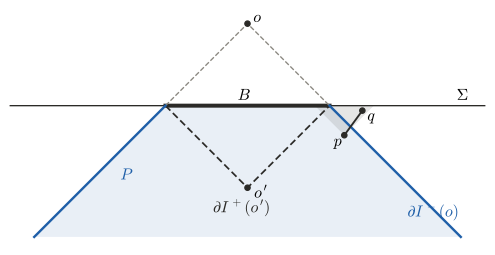
Figure 1. A section through the centre of the ball. The horizon $\partial I^-(o)$ is the past light cone of the top tip $o$, continued below $\Sigma$; $P$ is the region inside it. A molecule is a pair $p\prec q$ with $p\in P$ and $q$ outside; its type counts the other elements in the grey triangle $J^+(p)\cap I^-(\Sigma)$. The lower boundary of the diamond, $\partial I^+(o')$, is the second sheet discussed in section 7.

For an element $p\in P$ let $F(p)$ be the set of elements that lie to the past of $\Sigma$ and to the causal future of $p$, excluding $p$. A horizon molecule is a pair $p\prec q$ with $p\in P$ and $q\in F(p)$ outside $P$. Its type is $m=\lvert F(p)\rvert-1$, the number of elements of $F(p)$ other than $q$. A molecule of type 0 is Barton et al.’s horizon molecule: $q$ is the only element to the future of $p$ and the past of $\Sigma$, so $p\prec q$ is a link. (Their molecules with several upper elements, all outside the horizon, are a different family.) Given real weights $w_0,w_1,\dots$, the weighted count $H_w$ is the sum of $w_m$ over all molecules.

The expectation of $H_w$ is an integral over the position of the pair. Given $p$ and $q$, the remaining elements in $J^+(p)\cap I^-(\Sigma)$ form a Poisson process (the Slivnyak–Mecke property), so the probability that there are exactly $m$ of them is $(\rho V)^me^{-\rho V}/m!$, with $V(p)$ the volume of $J^+(p)\cap I^-(\Sigma)$. Writing $V_{\rm out}(p)$ for the volume of the part of this region outside $P$,

$$\langle H_w\rangle=\rho^2\int_P dV_p\;V_{\rm out}(p)\,\phi\big(\rho V(p)\big),\qquad \phi(v)=e^{-v}\sum_m w_m\frac{v^m}{m!}. \tag{1}$$

The weights enter only through the kernel $\phi$. We call

$$Q(\alpha)=\sum_m w_m\frac{(\alpha)_m}{m!},\qquad \Gamma(\alpha)\,Q(\alpha)=\int_0^\infty\phi(v)\,v^{\alpha-1}\,dv, \tag{2}$$

the Mellin symbol of the weighting; $(\alpha)_m=\alpha(\alpha+1)\cdots(\alpha+m-1)$, and the second equality follows from $\int_0^\infty v^{m+\alpha-1}e^{-v}dv/m!=\Gamma(\alpha)(\alpha)_m/m!$. Weights with $w_m=0$ for $m>N$ give a polynomial $Q$ of degree $N$. The weights are recovered from $Q$ through $(-j)_m/m!=(-1)^m\binom{j}{m}$ and binomial inversion:

$$w_m=\sum_{j=0}^{m}(-1)^j\binom{m}{j}\,Q(-j). \tag{3}$$

The type-0 count has $Q\equiv1$.

2. A weighting acts on the density dependence

The point of (2) is that weighting by $m$ is the same as acting on the dependence of the count on $\rho$.

Lemma 1 (density dependence). Fix the geometry and suppose that the type-0 count is a finite sum of powers of the density, $\langle H_{0}\rangle(\rho)=\sum_\beta C_\beta\,\rho^{2-\beta}$. Then for every weighting

$$\langle H_w\rangle(\rho)=\sum_\beta C_\beta\,Q(\beta)\,\rho^{2-\beta}. \tag{4}$$

Proof. Let $\mu$ be the measure on $(0,\infty)$ defined by $\int f\,d\mu=\int_P dV_p\,V_{\rm out}(p)\,f(V(p))$, so that $\langle H_w\rangle=\rho^2\int\phi(\rho V)\,d\mu(V)$, and let $L(\rho)=\int e^{-\rho V}d\mu(V)$, so that $\langle H_0\rangle=\rho^2L(\rho)$. Differentiating under the integral, $\int(\rho V)^me^{-\rho V}d\mu/m!=(-\rho)^mL^{(m)}(\rho)/m!$. On a power, $(-\rho)^m\partial_\rho^m\rho^{-\beta}/m!=\big((\beta)_m/m!\big)\rho^{-\beta}$. Summing over $m$ with weights $w_m$ gives (4).

In every case below the count is, order by order in the curvature, a polynomial in the size $\ell$ of the ball (this is part of the proof of Theorem 1), and dimensional analysis turns powers of $\ell$ into powers of $\rho$. The count is dimensionless and depends on $\rho$ only through $\rho\ell^d$ and $\rho$ times $d$-th powers of the curvature lengths. A term $\ell^e$ multiplying a curvature quantity of length dimension $-D$ therefore carries $\rho^{(e-D)/d}$, that is,

$$\beta=2-\frac{e-D}{d}. \tag{5}$$

For example, the flat area term $\ell^{d-2}$ has $D=0$ and $\beta=1+2/d$, which we call the area exponent $\alpha_A$. Equation (4) says that a weighting multiplies each term by its own number $Q(\beta)$. A weighting whose symbol vanishes at every $\beta$ except that of the leading term keeps only the term that survives as $\rho\to\infty$ at fixed $\ell$. This is Richardson extrapolation of the type-0 count to infinite density, carried out at a single density by using the information in $m$.

3. The flat count

From here on we set $\rho=1$, so lengths are in units of $\ell_\rho$. The computations below use one exact reduction, which holds for spacetimes conformal to a static one with round spatial sections. Let

$$g=W(t)^{2/d}\big(-dt^2+\gamma\big),$$

with $\gamma$ the round metric on the $n$-sphere of radius $A$ ($A=\infty$ gives flat space) and $W(0)=1$; the power $2/d$ makes the volume element $W\,dt\,dvol_\gamma$. Let $\Sigma=\{t=0\}$ and $B$ the geodesic ball of radius $r_0$ about a pole, and write $\mathrm{cap}(r)$ for the $\gamma$-volume of a geodesic ball of radius $r$ on the sphere.

Lemma 2 (reduction). With $\tau$ the coordinate depth of $p$ below $\Sigma$,

$$\langle H_w\rangle=\int_0^\infty d\tau\,W(-\tau)\,\phi\big(V(\tau)\big)\,U(\tau),\qquad U(\tau)=\int_0^\tau ds\,W(s-\tau)\,\mathrm{cap}(s)\big[\mathrm{cap}(r_0+\tau)-\mathrm{cap}(r_0+\tau-s)\big], \tag{6}$$

with $V(\tau)=\int_0^\tau ds\,W(s-\tau)\,\mathrm{cap}(s)$, as long as no cap wraps around the sphere (in particular to every order in $1/A$).

Proof. Conformal factors do not change causal relations, so $(t_1,y_1)\prec(t_2,y_2)$ exactly when the $\gamma$-distance from $y_1$ to $y_2$ is at most $t_2-t_1$. The tip $o$ sits at $t=r_0$ above the pole, so $P$ at time $-\tau$ is the cap $C_1$ of radius $r_0+\tau$ about the pole, and $V(p)$ depends only on $\tau$. An element $q$ at time $-(\tau-s)$ is to the future of $p=(-\tau,y_p)$ and outside $P$ when it lies in the cap of radius $s$ about $y_p$ and outside the cap $C_2$ of radius $r_0+\tau-s$ about the pole. Integrating over $y_p\in C_1$, the volume of the cap about $y_p$ gives $\mathrm{cap}(s)\,\mathrm{cap}(r_0+\tau)$. In the part inside $C_2$ we exchange the roles of $y_p$ and $y_q$: for $y_q\in C_2$ the cap of radius $s$ about $y_q$ lies inside $C_1$ by the triangle inequality, so this part is $\mathrm{cap}(s)\,\mathrm{cap}(r_0+\tau-s)$.

In flat space $W=1$ and $\mathrm{cap}(r)=\omega r^n$, with $\omega$ the volume of the unit $n$-ball. Then $V=\omega\tau^d/d$, and expanding the bracket in (6) binomially in $\ell=r_0$, the term of order $\ell^n$ cancels:

$$U(\tau)=\omega^2\sum_{k=1}^{n}\binom nkI_k\,\ell^{\,n-k}\tau^{d+k},\qquad I_k=\int_0^1\zeta^n\big[1-(1-\zeta)^k\big]d\zeta=\frac1d-\frac{n!\,k!}{(n+k+1)!}.$$

Substituting $v=\omega\tau^d/d$ turns each $\tau$-integral into (2).

Proposition 1 (flat count). For a flat ball of radius $\ell$,

$$\langle H_w\rangle=\sum_{k=1}^{n}\binom nkI_k\,\frac{\omega^2}{d}\Big(\frac d\omega\Big)^{\beta_k}\Gamma(\beta_k)\,Q(\beta_k)\,\ell^{\,n-k},\qquad\beta_k=\frac{d+1+k}{d}. \tag{7}$$

There is no term proportional to $\ell^{n}$, the volume of $B$. The leading term is $Q(\alpha_A)\,a_d\,\lvert\partial B\rvert$, with $\lvert\partial B\rvert=n\omega\ell^{n-1}$ and

$$a_d=\frac{\omega}{d(d+1)}\Big(\frac d\omega\Big)^{\alpha_A}\Gamma(\alpha_A). \tag{8}$$

The proof is the computation above; $I_1=1/(d+1)$ gives (8). The exponents present are $\alpha_A,\alpha_A+\tfrac1d,\dots,2$. Equation (8) gives $a_3=\tfrac14(3/\pi)^{2/3}\Gamma(5/3)=0.218853$ and $a_4=\sqrt3/10$, the coefficients found by Barton et al., and $a_5=0.148656$, $a_6=0.133258$. In four dimensions,

$$\langle H_w\rangle=\frac{2\sqrt3\,\pi}{5}\,Q(\tfrac32)\,\ell^2+\frac{7\cdot3^{3/4}\pi^{1/4}\Gamma(\frac34)}{10}\,Q(\tfrac74)\,\ell+\frac{34}{35}\,Q(2). \tag{9}$$

For the type-0 count ($Q\equiv1$) this is $2.17656\,\ell^2+2.60322\,\ell+0.97143$. A direct sprinkling agrees with (9) for each type separately: at $\ell=1$ the mean counts of types 0, 1, 2 over 600 sprinklings are $5.78\pm0.11$, $9.78\pm0.18$, $13.15\pm0.24$, against $5.751$, $9.763$, $13.259$ from (9), and at $\ell=6$ the type-0 count is $95.4\pm1.3$ (60 sprinklings) against $94.95$. The linear term of (9) differs from the first correction given by Barton et al.; the comparison is made in section 7, where the sheet used in their calculation appears.

4. Curvature response of a ball of fixed volume

In curved space we hold the volume of $B$ fixed at $\omega\ell^n$, so that $\ell$ labels its size, and expand in the curvature. In the class of Lemma 2 the term of $\langle H_w\rangle$ at the area exponent is the exact area of $\partial B$, to all orders.

Theorem 1 (area exponent). In the setting of Lemma 2, with $W$ analytic, $W(0)=1$, and $B$ of fixed volume $\omega\ell^n$, expand $\langle H_w\rangle$ as a formal power series in $1/A^2$ and in the Taylor coefficients of $W$. Each coefficient is a polynomial in $\ell$. At every order, the term multiplying $Q(\alpha_A)$ is $a_d\,Q(\alpha_A)$ times the corresponding term of $\lvert\partial B\rvert$, the area of the boundary of the fixed-volume ball. All other terms carry $Q$ at points $\alpha_A+j/d$ with $j\ge1$.

The idea is that $\ell$ enters (6) only through $r_0$ inside the bracket. At each order the highest power of $\ell$ comes from the first derivative $\mathrm{cap}'(r_0)$ with every other factor at its flat value, and $\mathrm{cap}'(r_0)$ is the area of $\partial B$.

Proof. Expand the bracket in (6) as $\sum_{i\ge1}\mathrm{cap}^{(i)}(r_0)\,[\tau^i-(\tau-s)^i]/i!$. The cap volume is a series $\sum_\nu\omega_\nu A^{-2\nu}r^{n+2\nu}$ with $\omega_0=\omega$, and the fixed-volume condition gives $r_0=\ell\,\psi(\ell^2/A^2)$ for a power series $\psi$; hence the order-$A^{-2\nu}$ part of $\mathrm{cap}^{(i)}(r_0)$ is a constant times $\ell^{\,n+2\nu-i}$. No other factor in (6), nor the expansion of $\phi(V)$ about $\omega\tau^d/d$, involves $\ell$, and the $s$- and $\tau$-integrals of the resulting monomials are finite. So each coefficient is a polynomial in $\ell$. Consider a term of order $A^{-2\nu}$ that also contains Taylor coefficients of $W$ of total length dimension $-D'$ (the coefficient of $t^k$ has dimension $-k$). Its power of $\ell$ is at most $n-1+2\nu$, so by (5) with $D=2\nu+D'$ its exponent is at least $2-(n-1-D')/d=\alpha_A+D'/d$. Equality requires $D'=0$, $i=1$, and the flat values of $\mathrm{cap}(s)$ and $V$. That term is $[\mathrm{cap}'(r_0)]_{\nu}\int_0^\infty d\tau\,\phi(\omega\tau^d/d)\int_0^\tau ds\,\omega s^{n}\,s$, which by the flat computation equals $a_d\,Q(\alpha_A)\,[\mathrm{cap}'(r_0)]_\nu$. Finally $\mathrm{cap}'(r_0)=\lvert\partial B\rvert$. All other terms have $\beta>\alpha_A$, and by (5) $\beta$ lies on the lattice $\alpha_A+j/d$.

At linear order and for curvature that is uniform over the diamond, two backgrounds suffice. The Einstein static universe ($W=1$) has spatial scalar curvature $R^\Sigma=n(n-1)/A^2$ and $R_{uu}=0$, with $u$ the unit normal to $\Sigma$. De Sitter space in conformal time ($W=\cos^{-d}(t/A)$) has the same slice and $R_{uu}=-n/A^2$. On a slice with vanishing extrinsic curvature, the linear response is a rotation-invariant linear function of the Riemann tensor at the centre, and the only such scalars are $R^\Sigma$ and $R_{uu}$: the Weyl tensor enters through $C_{uiuj}$, which is traceless and averages to zero over directions. This reduction rests on rotation invariance. We write the response at fixed volume as

$$\delta\langle H_w\rangle\big|_V=-h_\Sigma(\ell)\,R^\Sigma-h_0(\ell)\,R_{uu}. \tag{10}$$

A geodesic sphere of radius $r$ has area $n\omega r^{n-1}\big(1-R^\Sigma r^2/(6n)\big)$ and encloses volume $\omega r^n\big(1-R^\Sigma r^2/(6(n+2))\big)$ at first order in the curvature at its centre. Eliminating $r$ at fixed volume gives $\delta\lvert\partial B\rvert_V=-c_d\,\ell^d R^\Sigma$ with $c_d=\omega/(2(d+1))$ ($c_4=2\pi/15$), the deficit used by Jacobson [Jacobson 2015]. By Theorem 1 the part of $h_\Sigma$ at $\alpha_A$ is $a_dQ(\alpha_A)c_d\ell^d$. And $h_0$, obtained from the difference between de Sitter and the static universe, has no part at $\alpha_A$, because the two have the same slice and the same ball. By (5) with $D=2$, a term $\ell^e$ in $h_\Sigma$ or $h_0$ carries $Q(2+(2-e)/d)$.

The remaining coefficients follow from (6) by expanding to first order in $1/A^2$: $\mathrm{cap}(r)=\omega r^n\big(1-\tfrac{n(n-1)}{6(n+2)}r^2/A^2\big)$, $r_0=\ell\big(1+\tfrac{n-1}{6(n+2)}\ell^2/A^2\big)$ from the fixed-volume condition, and $W=1+\tfrac d2t^2/A^2$ for de Sitter. Each monomial in $\tau$ is then integrated with (2), and a term $\phi'$ from the change of $V$ gives $\int v^{b-1}\phi'\,dv=-\Gamma(b)Q(b-1)$. For example, in four dimensions the $\ell^2$ term of $h_0$ comes from the $\omega\cdot3\ell^2s$ term of the bracket and from the three places where de Sitter’s $W$ enters: $W(-\tau)$, $W(s-\tau)$ in $U$, and the change of $V$. These contribute $\tfrac{24}{5}$, $\tfrac{8}{35}$ and $-\tfrac{16}{25}$ times $Q(2)$, and dividing their sum by $d-1=3$ (from $R_{uu}=-3/A^2$) gives $\tfrac{256}{175}Q(2)$. In four dimensions the result is the following table: each response is the sum of the entries in its column, and each entry is multiplied by $Q$ at the exponent in the first column.

exponent $\alpha$	flat count	$h_\Sigma$	$h_0$
$3/2$	$\frac{2\sqrt3\pi}{5}\ell^2$	$\frac{\sqrt3\pi}{75}\ell^4$	$0$
$7/4$	$\frac{7\cdot3^{3/4}\pi^{1/4}\Gamma(3/4)}{10}\ell$	$\frac{7\cdot3^{3/4}\pi^{1/4}\Gamma(3/4)}{100}\ell^3$	$0$
$2$	$\frac{34}{35}$	$\frac{48}{175}\ell^2$	$\frac{256}{175}\ell^2$
$9/4$		$\frac{31\cdot3^{1/4}\Gamma(1/4)}{1120\,\pi^{1/4}}\ell$	$\frac{37\cdot3^{1/4}\Gamma(1/4)}{70\,\pi^{1/4}}\ell$
$5/2$		$\frac{\sqrt3}{1260}$	$\frac{547\sqrt3}{1260}$

The first entry of $h_\Sigma$ is $a_4c_4\ell^4$, as Theorem 1 requires. We computed the same tables exactly in $d=3,\dots,8$. In each, $h_\Sigma$ has nonzero coefficients at all $d+1$ exponents $\alpha_A+j/d$, $j=0,\dots,d$, $h_0$ at $j=2,\dots,d$, and the flat count at $j=0,\dots,d-2$; every coefficient is positive. Two independent calculations agree on the four-dimensional table.

5. The linearised Einstein equation with the area-law coefficient

We take the following model, which is Jacobson’s setting [Jacobson 2015] with a causal-set count in place of the entanglement entropy of the short-distance degrees of freedom.

1. The short-distance entropy of the diamond over $B$ is $s_0\langle H_w\rangle$ for a constant $s_0$ (for instance $\ln2$ per molecule). Only the expected count enters; fluctuations are ignored.
2. In flat space this entropy defines Newton’s constant through $S=\lvert\partial B\rvert/4G$ at leading order, so $1/(4G)=s_0\,Q(\alpha_A)\,a_d\,\rho^{(d-2)/d}$.
3. Entanglement equilibrium holds: at fixed volume the change of the short-distance entropy balances the change of the matter entropy.

In Jacobson’s argument the balance in item 3, imposed for every unit timelike $u$, is equivalent to the Einstein equation with coupling $G_N$ when the short-distance entropy changes by $\delta\lvert\partial B\rvert_V/4G_N$; on a slice with vanishing extrinsic curvature the Gauss equation gives $R^\Sigma=2G_{uu}$, so that $\delta\lvert\partial B\rvert_V=-2c_d\ell^dG_{uu}$. Comparing with (10), the count gives the linearised Einstein equation with $G_N=G$ at every size $\ell$ exactly when

(i) $h_0(\ell)=0$, and (ii) $h_\Sigma(\ell)=Q(\alpha_A)\,a_d\,c_d\,\ell^d$.

If (i) fails, the response depends on $R_{uu}$ separately and the equation is not Einstein’s. For matter with $R_{uu}=\lambda R^\Sigma$ the balance then defines an effective $G_N/G=Q(\alpha_A)a_dc_d\ell^d/(h_\Sigma+\lambda h_0)$; in four dimensions, under the Einstein equation, $\lambda=1/4$ for dust and $1/2$ for radiation.

For the type-0 count the table gives $G_N/G=1/(1+3.59/\ell+3.78/\ell^2+\dots)$ for $\lambda=0$, so for $\ell\gg\ell_\rho$ both conditions hold up to relative corrections of order $\ell_\rho/\ell$. The conditions matter for diamonds a few discreteness lengths across. As an illustration, take the diamonds spanned by links. A diamond of half-height $\ell$ has volume $2\pi\ell^4/3$ in four dimensions, and a related pair is a link when this diamond is empty, while the number of related pairs at proper time $2\ell$ grows as $T^{d-1}dT\propto\ell^3d\ell$, with $T=2\ell$ the proper time between the pair, per unit boost volume, so the half-heights of links are distributed as $\ell^3e^{-2\pi\ell^4/3}$. Averaging the numerator and denominator of $G_N/G$ over this distribution, the type-0 count gives $G_N/G=0.0832$, $0.0292$ and $0.0177$ for $\lambda=0$, dust and radiation. Other populations of sizes give other values.

Theorem 2 (exact weights). Let $d\ge3$ and let $w$ be a finite weighting with $Q(\alpha_A)\neq0$.

(a) If $Q(\alpha_A+j/d)=0$ for $j=1,\dots,d$, then for every $\ell>0$ the flat count is $Q(\alpha_A)a_d\lvert\partial B\rvert$ and conditions (i) and (ii) hold.

(b) For $3\le d\le8$, condition (ii) alone implies these $d$ zeros.

(c) A weighting with these zeros has $w_m\neq0$ for some $m\ge d$. Among weightings with $w_m=0$ for $m>d$ it is unique up to normalisation, with

$$Q_d(\alpha)=\binom{2d+2-d\alpha}{d},\qquad w_m=\sum_{j=0}^{m}(-1)^j\binom mj\binom{2d+2+dj}{d}. \tag{11}$$

Proof. (a) By (4) and the structure in section 4, the weighted flat count and $h_\Sigma$, $h_0$ are sums over $j$ of $Q(\alpha_A+j/d)$ times the type-0 coefficients, with $j\le d$. The zeros leave only $j=0$, which is $Q(\alpha_A)a_d$ times $\lvert\partial B\rvert$, times $c_d\ell^d$, and times zero respectively. (b) Condition (ii) says that $\sum_{j=1}^dC^\Sigma_j\,Q(\alpha_A+j/d)\,\ell^{d-j}$ vanishes identically in $\ell$, where $C^\Sigma_j$ are the type-0 coefficients of $h_\Sigma$; these are nonzero for $d\le8$. (c) If $w_m=0$ for $m>N$, $Q$ is a polynomial of degree at most $N$, so $d$ zeros require $N\ge d$ unless $Q\equiv0$; for $N=d$ it is fixed up to a constant by its zeros. With $z=2d+2-d\alpha$, $\binom zd$ vanishes at $z=0,\dots,d-1$, which are the points $\alpha=\alpha_A+j/d$, $j=d,\dots,1$, and equals 1 at $z=d$, which is $\alpha=\alpha_A$. The weights follow from (3).

Part (a) covers general uniform curvature through the rotation-invariance reduction of section 4. The weights are integers, with $w_0=\binom{2d+2}{d}$ and $w_d=(-d)^d$:

$d$	zeros of $Q_d$	weights $w_0,\dots,w_d$	$a_d$
3	$2,\ \tfrac73,\ \tfrac83$	$56,\ -109,\ 90,\ -27$	$0.218853$
4	$\tfrac74,\ 2,\ \tfrac94,\ \tfrac52$	$210,\ -791,\ 1268,\ -928,\ 256$	$0.173205$
5	$\tfrac85,\dots,\tfrac{12}5$	$792,\ -5396,\ 14750,\ -19500,\ 12500,\ -3125$	$0.148656$
6	$\tfrac32,\dots,\tfrac73$	$3003,\ -35757,\ 155713,\ -328779,\ 365256,\ -206064,\ 46656$	$0.133258$

We checked with the exact responses that these weights give a flat count equal to $a_d\lvert\partial B\rvert$, $h_\Sigma=a_dc_d\ell^d$ and $h_0=0$ identically in $\ell$, in $d=3,\dots,8$. With more than $d+1$ weights there are $N-d$ free parameters; “unique” means unique at minimal degree.

Given Theorem 1, every weighting whose symbol vanishes at the $d$ non-area exponents satisfies (i) and (ii), whatever principle is used to choose it, and a weighting that keeps one of them fails. Keeping the exponent $\alpha=2$, for example, with $Q(2)=q\neq0$ and the other three zeros in four dimensions, gives $h_0=\tfrac{256}{175}q\,\ell^2$. The weights make the continuum statement hold without corrections in $\ell_\rho/\ell$; the statement itself comes from the locality of the count.

Remark (relation to the causal-set d’Alembertian). The four-dimensional d’Alembertian of Benincasa and Dowker [BD] uses the same kind of kernel, a polynomial times $e^{-v}$, with layer coefficients $(1,-9,16,-8)$; by (2) its Mellin symbol vanishes at $\alpha=\tfrac12,1,\tfrac32$. These zeros are spaced by $2/d$, and they serve to make the continuum limit the local operator $\Box$. The zeros of $Q_d$ are spaced by $1/d$, lie above the exponent that is kept, and remove the finite-density corrections to a limit that is already local.

As a combinatorial aside, $Q_d(\alpha)=b(\alpha_A-\alpha)/b(0)$ with $b(s)=\prod_{j=1}^d(s+j/d)$ the Bernstein–Sato polynomial of $x^d$, and $Q_d$ is the Ehrhart polynomial of the standard $d$-simplex evaluated at $d+2-d\alpha$.

6. Signs, minimal degree and the cost of cancellation

Proposition 2 (no nonnegative weighting). If $\phi\ge0$ and $\phi\not\equiv0$, in particular if every $w_m\ge0$, then $Q(\alpha)>0$ for all $\alpha>0$, and no zero required in Theorem 2 can occur. For $3\le d\le8$, moreover, $h_0(\ell)>0$ and $h_\Sigma(\ell)>Q(\alpha_A)a_dc_d\ell^d$ for every $\ell$, so that $G_N<G$ for every $\lambda\ge0$, at every size and for every population of sizes.

Proof. The first statement is (2). The second follows because $h_0$ and $h_\Sigma-Q(\alpha_A)a_dc_d\ell^d$ are sums of positive coefficients times positive values $Q(\alpha_A+j/d)$ (section 4).

For the caustic-free sheet, at linear order and for uniform curvature, an entropy that counts molecules with a positive amount each therefore gives a weaker gravitational coupling than its own area law at finite density ($d\le8$, $\lambda\ge0$). Signed weights are required, and the number of sign changes of $\phi$ is bounded below by the number of zeros of $Q$. The following lemma is classical; its proof is short.

Lemma 3 (sign changes). Let $\phi$ be continuous on $(0,\infty)$ with finitely many sign changes, and suppose $\int_0^\infty\phi(v)v^{\alpha_k-1}dv=0$, with absolute convergence, for $Z$ distinct real $\alpha_k$. Then $\phi\equiv0$ or $\phi$ changes sign at least $Z$ times.

Proof. Suppose $\phi$ changes sign exactly at $v_1<\dots<v_r$ with $r<Z$. A nonzero combination $\sum_{k=1}^{r+1}c_kv^{\alpha_k-1}$ has at most $r$ positive zeros counted with multiplicity (Descartes’ rule for generalised polynomials), and the $r$ conditions that it vanish at the $v_i$ have a nonzero solution. That solution changes sign exactly at the $v_i$, so its product with $\phi$ has one sign. Its integral is zero by hypothesis, so $\phi\equiv0$.

Corollary 1 (alternation). If $w_m=0$ for $m>N$ and $Q$ vanishes at $N$ positive points, then $w_0,\dots,w_N$ are all nonzero and strictly alternate in sign. In particular the weights (11) alternate.

Proof. By Lemma 3, $\phi=e^{-v}p(v)$ with $p(v)=\sum w_mv^m/m!$ changes sign at least $N$ times, so $p$ has at least $N$ positive zeros. By Descartes’ rule its $N+1$ coefficients then have at least $N$ sign changes, which forces every coefficient to be nonzero and the signs to alternate.

The area term survives a large cancellation. In four dimensions $\phi_4(v)=e^{-v}\big(210-791v+634v^2-\tfrac{464}{3}v^3+\tfrac{32}{3}v^4\big)$ changes sign at $v\approx0.36,\ 1.58,\ 4.05,\ 8.5$ and ranges between $-41.8$ and $210$. The area term is the moment $\int\phi_4v^{1/2}dv/\Gamma(\tfrac32)=1$, while $\int\lvert\phi_4\rvert v^{1/2}dv/\Gamma(\tfrac32)=114.9$. For the symbols $Q=\binom{N+6-4\alpha}{N}$, which cancel $N$ exponents, this ratio is $929$, $7.2\times10^3$ and $4.0\times10^5$ for $N=6$, $8$, $12$, about a factor $2.8$ per additional zero. The weights themselves grow at least geometrically: from $Q(-j)=\sum_mw_m(-1)^m\binom jm$ one gets $\sum_m\lvert w_m\rvert\ge Q(-j)/2^j$ for every $j$, and $j=N$ gives $\sum_m\lvert w_m\rvert\ge\binom{5N+6}{N}2^{-N}$, which grows like $6.1^N$. Poisson fluctuations of $H_w$ are amplified by the same cancellation.

7. Scope: gradients, orientation and non-linear order

Gradients of the curvature

Theorem 2 concerns curvature that is uniform over the diamond. Gradients add exponents beyond $\alpha_A+1$. The class of Lemma 2 contains time-dependent examples: $W=e^{d\,\varepsilon_kt^k}$ with $k\ge2$ is conformally flat, its slice $t=0$ is flat with vanishing extrinsic curvature, and for $k=3$ the scalar curvature vanishes on $\Sigma$ while its time derivative does not. At first order in $\varepsilon_k$ the count is a polynomial in $\ell$ of degree $d-2$, and by (5) its terms sit at the exponents $\alpha_A+k/d,\dots,2+k/d$. For $k=3$ the $Q_d$-weighted count does not vanish:

$$\frac{2511}{175\pi}\,\varepsilon_3\quad(d=3),\qquad -\frac{3377\cdot3^{3/4}\Gamma(\frac34)}{700\,\pi^{3/4}}\,\varepsilon_3\approx-5.71\,\varepsilon_3\quad(d=4),$$

in units $\rho=1$, while the area of $\partial B$ does not change. Theorem 2 therefore holds for sources without gradients, and a first time derivative of the scalar curvature already leaves a residual at linear order.

At the next order in gradients the exponents run up to $\alpha_A+(d+2)/d$. The symbol $\binom{2d+4-d\alpha}{d+2}$ removes them; in four dimensions its weights are

$$(924,\,-7084,\,23668,\,-41416,\,39808,\,-19968,\,4096).$$

With these weights the $k=3$ and $k=4$ responses above vanish identically in $d=3$ and $d=4$. Each order in gradients needs new weights. The first exponent that a weighting does not cancel enters with $\lvert Q_d\rvert\ge1$, at least as large as in the type-0 count: $Q_d(\alpha_A+(d+k)/d)=(-1)^d\binom{d+k-1}{d}$, which is $\pm1$ for $k=1$.

Orientation of the horizon sheet

Two null sheets pass through $\partial B$ below $\Sigma$ (Figure 1). The one used so far, $\partial I^-(o)$, moves away from $B$ into the past. The other is the lower boundary of the diamond itself, $\partial I^+(o')$ with $o'$ the bottom tip; it contracts into the past and has a caustic at $o'$, a depth $\ell$ below $\Sigma$. Molecules are defined for it in the same way, with $p$ outside $I^+(o')$ and $q$ inside. Barton et al. define molecules for horizons of the first kind. In flat four-dimensional space, the argument of Lemma 2 applies to the second sheet with the bracket replaced by $\mathrm{cap}(\ell-\tau+s)-\mathrm{cap}(\ell-\tau)$, caps of negative radius being empty. For $\tau<\ell$ this is the bracket of the first sheet evaluated at $-\ell$, since $\mathrm{cap}(r)=\omega r^3$ is odd. Hence

$$\langle H_w\rangle_{\rm lower}(\ell)=\langle H_w\rangle(-\ell)-\mathcal D_w(\ell),$$

where $\langle H_w\rangle(-\ell)$ is the polynomial (9) evaluated at $-\ell$ and the defect $\mathcal D_w$ comes from molecules whose lower element lies below the caustic. Write $\sigma=\tau-\ell$ for the depth of $p$ below $o'$. For each type,

$$\mathcal D_m(\ell)=\int_0^\infty d\sigma\;\frac{V^m e^{-V}}{m!}\Big|_{V=\pi(\ell+\sigma)^4/3}\;\frac{4\pi^2}{315}\,\sigma^3\big(35(\ell+\sigma)^4-\sigma^4\big)>0,$$

where the polynomial is the difference between the continued bracket of the first sheet and the true bracket of the second, integrated over $s$. Laplace’s method gives $\mathcal D_m(\ell)=\frac{27}{32\pi^2}\frac{(\pi\ell^4/3)^m}{m!}\ell^{-8}e^{-\pi\ell^4/3}\big(1+O(\ell^{-4})\big)$; we checked the asymptotic form numerically to $2\times10^{-4}$ at $\ell=12$. Here $\pi\ell^4/3$ is the volume of the half of the diamond below $\Sigma$, which lies to the future of every $p$ below the caustic.

Proposition 3 (no exact weighting for the lower sheet). In flat four-dimensional space no finite nonzero weighting makes the count across the lower sheet proportional to $\ell^2$ for all $\ell>0$.

Proof. If it did, $\mathcal D_w(\ell)$ would equal a polynomial in $\ell$, and since $\mathcal D_w$ tends to zero faster than any power, the polynomial and $\mathcal D_w$ would vanish identically. But if $M$ is the largest $m$ with $w_m\neq0$, the asymptotic form shows $\mathcal D_w(\ell)\sim w_M\mathcal D_M(\ell)\neq0$ for large $\ell$.

For the weights of Theorem 2 and $\ell\ge2.2\,\ell_\rho$ the defect is below $10^{-7}$ of the area term. The reflection also holds for the curvature responses of section 4, since in $d=4$ every cap volume is odd in its radius; reflecting $\ell$ changes no exponent, so $Q_4$ gives the area law and conditions (i) and (ii) on this sheet as well for such sizes. At smaller sizes it does not. With the weights of Theorem 2 the flat count across the lower sheet, divided by $a_4\lvert\partial B\rvert$, is $1.113$, $0.959$ and $0.99998$ at $\ell=1$, $1.36$ and $1.9$, and $h_0$ is $-0.253$, $-0.364$ and $-8\times10^{-5}$. Averaged over the link population of section 5, $G_N/G=1.350$, $8.450$ and $-1.984$ for $\lambda=0$, dust and radiation; the negative value means that for radiation the count’s response has the opposite sign to the area’s. The caustic separates the two sheets. Reversing time maps the first sheet, counted to the past of $\Sigma$, to the future light cone of the bottom tip continued above $\Sigma$, counted to the future, and the same weights are exact there; the upper boundary of the diamond, counted to the future, has its caustic at $o$ and behaves like the lower sheet.

Remark (the first correction to the area law). Barton et al. write the first correction for the type-0 count as $b^{(4)}_{3,1}\,\theta\,\ell_\rho$ per unit area, with $\theta$ the expansion of the horizon at $\partial B$, and give $b^{(4)}_{3,1}=-\sqrt2\,\Gamma(\tfrac{11}4)/(35\cdot3^{1/4}\pi^{3/4})\approx-0.0209$ (their eq. 5.51). To calibrate $b^{(4)}_{3,1}$ they use, in a time-reversed set-up, the past light cone of a point whose cross-section with $\Sigma$ is a sphere of radius $r$; reversed back, this is the second sheet above, with $r=\ell$. With their normalisation of the null normal, $\theta=\sqrt2/\ell$. The second sheet carries the linear term of (9) with opposite sign, so (9) gives $b^{(4)}_{3,1}=-7\cdot3^{3/4}\Gamma(\tfrac34)/(40\sqrt2\,\pi^{3/4})\approx-0.1465$, exactly seven times their value. Their value is reproduced exactly by their integral $I_1$ built from the $V_+$ of their eq. (5.47) if the factor $(1+X^1/r)^2$ is set to one. Here $X^1$ is the coordinate of the lower element along the outward normal to $\partial B$ within $\Sigma$, measured from $\partial B$, and the factor is the ratio between the area of the sphere through that element and the area of $\partial B$. With the factor included the integral gives the value from (9). Their $I_n$ is defined in normal coordinates adapted to $\partial B$ but evaluated in Minkowski coordinates; the factor is the Jacobian between the two at first order, which is a likely origin of the difference. A sprinkling distinguishes the two values. For the second sheet at $\ell=6$, 60 sprinklings give $62.3\pm1.1$ type-0 molecules; the exact count is $63.7$, and their coefficient, with the constant term of (9), gives $77.1$.

Beyond linear order

Theorem 1 holds beyond linear order: in the class of Lemma 2 the term at the area exponent is the exact area of the fixed-volume ball to all orders in $1/A^2$ and in the derivatives of $W$, and with $Q_d$ every other term up to $j=d$ is removed. At second order in $1/A^2$ in $d=3$ the weighted count is

$$a_3\lvert\partial B\rvert+\frac{1}{A^4}\Big(\frac{27\,\ell}{560\pi}+\frac{2\cdot3^{1/3}\Gamma(\frac13)}{225\,\pi^{4/3}}\Big)\ \text{(static universe)},\qquad a_3\lvert\partial B\rvert-\frac{1}{A^4}\Big(\frac{17307\,\ell}{2800\pi}+\frac{4109\cdot3^{1/3}\Gamma(\frac13)}{450\,\pi^{4/3}}\Big)\ \text{(de Sitter)},$$

with residuals at $j=4,5$ only. The residuals are suppressed by $(\ell_\rho/\ell)^{d+1}$ relative to the area term but have large coefficients: in de Sitter the residual exceeds the second-order part of $a_3\lvert\partial B\rvert$, which is $-0.0107\,\ell^5/A^4$, for $\ell<4.3\,\ell_\rho$.

This does not by itself give the non-linear Einstein equation. When $W'(0)\neq0$ the slice $t=0$ has extrinsic curvature $K_{ij}\propto\gamma_{ij}$, the area deficit of $B$ follows $R^\Sigma$, and by the Gauss equation $R^\Sigma=2G_{uu}-(K^2-K_{ij}K^{ij})\neq2G_{uu}$. Jacobson’s argument uses, for each point $x$ and unit timelike $u$, geodesic balls in the slice $\Sigma_u$ generated by geodesics orthogonal to $u$ at $x$, whose extrinsic curvature vanishes at $x$. In an expanding universe these slices are not of the form $t=$ const, and Lemma 2 does not reach them. The non-linear statement is therefore conditional on the following property.

(J) For every $x$ and $u$, and for geodesic balls $B\subset\Sigma_u$ with $\ell_\rho\ll\ell\ll L$, $L$ the curvature length, the term of the count at the area exponent is $a_d$ times the area of $\partial B$.

If (J) holds, the count supplies $\delta S=\delta\lvert\partial B\rvert_V/4G$, where at leading order in $\ell/L$, $\delta\lvert\partial B\rvert_V=-2c_d\ell^dG_{uu}$ for all $u$. Jacobson’s argument then gives $G_{ab}+\Lambda g_{ab}=8\pi G\,T_{ab}$, including its non-linear terms, with $\Lambda$ an integration constant that the argument leaves undetermined. (J) is supported by the locality of the leading term of the count [Barton et al.] and by a flat-space property: the coefficient of a corner, a null plane meeting a spacelike hyperplane in a codimension-two plane, does not depend on the tilt of the hyperplane. A boost along the null plane maps one tilted hyperplane through the corner to any other and preserves the sprinkling, the order and all volumes. Curvature, the extrinsic curvature of $\Sigma_u$ and that of $\partial B$ enter at $j\ge1$ by (5), where $Q_d$ removes them up to $j=d$. Property (J) has not been verified by computing the count on a curved slice $\Sigma_u$. Even if it holds, the count supplies only the entropy term. The first law for the matter, the conformal Killing vector of the diamond and the vacuum-state hypothesis remain Jacobson’s assumptions, and the temperature and heat flux are not derived from the causal set.

8. Exactness to all orders and slowly decaying kernels

A weighting of finite degree $N$ cancels at most $N$ exponents, by Lemma 3, because $e^{-v}p(v)$ with $p$ of degree $N$ changes sign at most $N$ times. Every order in gradients adds new exponents. In the time-dependent family of section 7 the $\ell^0$ term of the $\varepsilon_k$-response sits at $2+k/d$, and its coefficient is nonzero for every $k=2,\dots,8$ in $d=3$ and $d=4$; together with section 4 this covers $\alpha_A+j/d$ for $1\le j\le10$ in four dimensions and $1\le j\le9$ in three. We assume this continues.

(H) For every $j\ge1$ some linear response in the class of Lemma 2 has a nonzero type-0 coefficient at $\alpha_A+j/d$.

Under (H), exactness to all orders means $Q(\alpha_A+j/d)=0$ for all $j\ge1$ with $Q(\alpha_A)\neq0$. Weightings by $m$ give kernels of the form $\phi(v)=e^{-v}\sum w_mv^m/m!$; we state the next result for general kernels $\phi$ on $(0,\infty)$, with $Q$ defined by (2), and use the length variable $x=v^{1/d}$, which is of the order of the proper-time extent of $J^+(p)\cap I^-(\Sigma)$ in units of $\ell_\rho$.

Theorem 3 (decay threshold). Let $\phi$ be bounded on $(0,1)$ with $\lvert\phi(v)\rvert\le C\exp(-c\,v^{1/(2d)})$ for $v\ge1$ and some $c,C>0$. If $Q(\alpha_A+j/d)=0$ for all $j\ge j_0$, then $\phi=0$ almost everywhere. Conversely, for every $\theta_0<1/(2d)$ there is a continuous $\phi$ with $\lvert\phi(v)\rvert\le C\exp(-c\,v^{\theta_0})$ such that $Q(\alpha_A+j/d)=0$ for all $j\ge1$ and $Q(\alpha_A)\neq0$.

In the variable $x$ the conditions are vanishing moments, and the threshold $e^{-c\sqrt x}$ is the classical boundary of determinacy for the Stieltjes moment problem on the half-line.

Proof. Put $\chi(x)=\phi(x^d)$. By (2), $\Gamma(\alpha)Q(\alpha)=d\int_0^\infty\chi(x)\,x^{d\alpha-1}dx$, and $d\alpha-1=d+1+j$ at $\alpha=\alpha_A+j/d$. So the hypothesis says $\int_0^\infty\chi(x)x^idx=0$ for all integers $i\ge i_0=d+1+j_0$, and $\lvert\chi(x)\rvert\le Ce^{-c\sqrt x}$ for $x\ge1$. Let $\chi_0(x)=x^{i_0}\chi(x)$, so that all moments of $\chi_0$ vanish, and define the even function $f_0(y)=\lvert y\rvert\chi_0(y^2)$ on $\mathbb R$. Substituting $x=y^2$ gives $\int_{\mathbb R}f_0(y)y^{2i}dy=\int_0^\infty\chi_0(x)x^idx=0$, and the odd moments vanish by symmetry. Since $\lvert f_0(y)\rvert\le C'e^{-c\lvert y\rvert/2}$, its Fourier transform $\hat f_0(\eta)$ is analytic in the strip $\lvert{\rm Im}\,\eta\rvert<c/2$, and its Taylor coefficients at $\eta=0$ are the moments of $f_0$, all zero. Hence $\hat f_0$ vanishes, $f_0=0$ and $\phi=0$ almost everywhere.

For the converse let $0<\kappa<\tfrac12$ and $f_1(x)=e^{-x^\kappa\cos\pi\kappa}\sin(x^\kappa\sin\pi\kappa)$. Substituting $t=x^\kappa$ and using $\int_0^\infty t^{a-1}e^{-t\cos\vartheta}\sin(t\sin\vartheta)\,dt=\Gamma(a)\sin(a\vartheta)$ for $\lvert\vartheta\rvert<\pi/2$ gives $\int_0^\infty f_1(x)x^{z-1}dx=\Gamma(z/\kappa)\sin(\pi z)/\kappa$, which vanishes at every positive integer $z$ (Stieltjes’ example). Let $f_2(x)=x^{-(d+2)}\int_x^\infty t^{d+1}f_1(t)\,dt$. By Fubini, $\int_0^\infty f_2(x)x^{z-1}dx=\Gamma(z/\kappa)\sin(\pi z)/(\kappa(z-d-2))$. This vanishes at $z=d+2+j$ for $j\ge1$ and equals $(-1)^d\pi\Gamma((d+2)/\kappa)/\kappa\neq0$ at $z=d+2$. The function $f_2$ is continuous on $[0,\infty)$ (the integral from 0 to $\infty$ of $t^{d+1}f_1$ vanishes, so $f_2(x)=O(x^{\kappa})$ near 0) and decays like $x^{-\kappa}e^{-x^\kappa\cos\pi\kappa}$. Then $\phi(v)=f_2(v^{1/d})/d$ has $\Gamma(\alpha)Q(\alpha)=\int_0^\infty f_2(x)x^{d\alpha-1}dx$, so it has the required zeros and $Q(\alpha_A)\neq0$, and it decays like $\exp(-c\,v^{\kappa/d})$. Take $\kappa=d\theta_0$.

The theorem covers exponentially decaying kernels, kernels supported on a bounded range of $v$ (a band in the volume variable), and weights with $\lvert w_m\rvert\le Cr^m$ for some $r<1$, which give $\lvert\phi(v)\rvert\le Ce^{-(1-r)v}$; none of these is exact to all orders. (For exponentially decaying kernels the same conclusion follows from Carlson’s theorem applied to $Q$.) Lemma 3 adds a second, independent condition: an exact kernel changes sign infinitely often. Decay and oscillation are separate requirements. A positive kernel can have a heavy tail, and $e^{-v}\sin v$ oscillates but decays exponentially. Kernels with finitely many sign changes, for example any finite combination of polynomials, exponentials and logarithms, are exact only to finite order, and for some the order is explicit.

Proposition 4 (exponential polynomials). A nonzero kernel $\phi(v)=\sum_{i=1}^{q}p_i(v)e^{-\mu_iv}$ with distinct $\mu_i>0$ and $\deg p_i\le N_i$ makes $Q$ vanish at no more than $\sum_i(N_i+1)-1$ positive points, and this number is attained with $Q(\alpha_A)\neq0$. For $q=1$, $\mu_1=1$ this is the bound $N$ for weights $w_0,\dots,w_N$.

Proof. A nonzero exponential polynomial of this form has at most $\sum_i(N_i+1)-1$ positive zeros: by induction on $q$, multiplying by $e^{\mu_qv}$ and differentiating $N_q+1$ times removes the last term and, by Rolle’s theorem, lowers the number of zeros by at most $N_q+1$. Lemma 3 then bounds the number of zeros of $Q$. To attain the bound, choose that many positive points different from $\alpha_A$ (for $\alpha>0$ the Mellin integrals converge); the linear conditions that $Q$ vanish there, on $\sum_i(N_i+1)$ coefficients, have a nonzero solution. If $Q(\alpha_A)$ also vanished, $Q$ would have $\sum_i(N_i+1)$ zeros, and by Lemma 3 $\phi$ would have more sign changes than it has positive zeros.

Theorem 3 describes how non-local an exact count must be. For the kernel of the proof with $\kappa=0.41$, the factor $e^{-x^\kappa\cos\pi\kappa}$ falls below $e^{-30}$ only at $x\approx9\times10^4$; in four dimensions $x\approx1.01\,\tau/\ell_\rho$, so molecules whose lower element lies some $10^5$ discreteness lengths below $\Sigma$ still contribute. The kernels of the proof are functions of $v$, whereas a weighting by $m$ gives $\phi(v)=e^{-v}\times$ (an entire function).

9. Open questions

The variance of the signed count is unknown, and the cancellation described in section 6 suggests that it is large. Responses to Weyl-type and transverse-traceless gradient sources have not been computed. Whether a weighting by $m$ alone, rather than a kernel in the continuum volume, can be exact to all orders in gradients is open.

References

1. Barton, Counsell, Dowker, Gould, Jubb, Taylor, “Horizon molecules in causal set theory,” arXiv:1909.08620.
2. Dou, Sorkin, “Black hole entropy as causal links,” arXiv:gr-qc/0302009.
3. Jacobson, “Entanglement equilibrium and the Einstein equation,” arXiv:1505.04753.
4. Benincasa, Dowker, “The scalar curvature of a causal set,” arXiv:1001.2725.
5. Dowker, Glaser, “Causal set d’Alembertians for various dimensions,” arXiv:1305.2588.
6. Glaser, “A closed form expression for the causal set d’Alembertian,” arXiv:1311.1701.
7. Aslanbeigi, Saravani, Sorkin, “Generalized causal set d’Alembertians,” arXiv:1403.1622.