Are Large Language Models (LLMs) just sophisticated statistical pattern matchers, or do they learn deeper linguistic structures? This post contributes to this ongoing debate by examining the information-theoretic efficiency of different approaches to modeling language. We investigate what the most efficient representation of language would look like from an information theory perspective, and whether learning such representations might be an inherent property of systems trained to predict language.

We’ll use the Minimum Description Length (MDL) principle to compare models with different levels of linguistic abstraction. Our thesis is that models incorporating principled linguistic structures (like syntactic categories and compositional rules) are fundamentally more efficient than purely statistical approaches. This suggests that LLMs, which are trained to optimize for predictive accuracy under size constraints, may be implicitly discovering and leveraging these structured abstractions rather than simply memorizing statistical patterns.

By analyzing a simple toy language through the lens of different modeling approaches, we’ll demonstrate how abstract linguistic structures lead to dramatic efficiency gains that become increasingly important as language complexity scales up. These findings offer insight into what LLMs might be “learning” when they achieve such remarkable performance on language tasks.

1. A Toy Model of Language

Let’s construct a tiny language to demonstrate our core concepts.

1.1 Lexicon and Categories

Our language has a small lexicon:

• Proper Nouns (PN): “Alice”, “Bob”
• Intransitive Verb (IV): “Dances”
• Transitive Verb (TV): “Calls”

For brevity, we represent these as: A = Alice (PN), B = Bob (PN), C = Calls (TV), D = Dances (IV).

These tokens belong to abstract categories, reflecting a basic ontological commitment (entities, actions, relations). This is our first layer of principled structure.

1.2 Syntactic Rules

A simple grammar defines how to build valid sentences:

1. $S \rightarrow PN \, IV$ (e.g., “Alice Dances”)
2. $S \rightarrow PN \, TV \, PN$ (e.g., “Alice Calls Bob”)

These rules are the second layer of principled structure.

1.3 Permissible Sentences

Using our lexicon and grammar, we can generate all permissible sentences:

1. From $S \rightarrow PN \, IV$:
   • “Alice Dances” (A D)
   • “Bob Dances” (B D)
2. From $S \rightarrow PN \, TV \, PN$:
   • “Alice Calls Alice” (A C A)
   • “Alice Calls Bob” (A C B)
   • “Bob Calls Alice” (B C A)
   • “Bob Calls Bob” (B C B)

There are exactly 6 permissible sentences in this toy language. Their lengths are 2 or 3 tokens.

Having established our toy language, we can now explore how different modeling approaches compare in their information efficiency.

2. Comparing Models with Minimum Description Length (MDL)

The MDL principle provides a formal framework for model comparison based on information efficiency. It states that the best model for a set of data is the one that minimizes the sum of:

1. The description length of the model itself ($L(\text{Model})$)
2. The description length of the data when encoded using the model ($L(\text{Data} \mid \text{Model})$)

For our comparison, we’ll examine models that perfectly generate our 6 sentences, meaning $L(\text{Data} \mid \text{Model}) = 0$. This allows us to directly compare $L(\text{Model})$ for different approaches.

Assume our four linguistic tokens (A, B, C, D) can each be uniquely identified with 2 bits (e.g., A=00, B=01, C=10, D=11).

2.1 Model 0: Unstructured Statistical Enumeration

This model describes the set of 6 permissible sentences by simply listing them without leveraging any linguistic abstractions.

• The sentences are: A D, B D, A C A, A C B, B C A, B C B.
• Total linguistic tokens: 16. Cost of tokens: $16 \times 2 = 32$ bits.
• To specify sentence structure by listing the tokens and their grouping, we also need to delimit sentences. One way is to provide the sequence of tokens and then specify the length of each of the 6 sentences. Each length (2 or 3) needs 2 bits (we need 2 bits because we need to distinguish between multiple possible lengths - 01 for length 2, 10 for length 3 - using a prefix-free code for lengths). So, $6 \times 2 = 12$ bits for lengths.
• Thus:

$$L(\text{Model}_0) = L(\text{Rote List}) \approx 32 \text{ (tokens)} + 12 \text{ (lengths)} = 44 \text{ bits}$$

This $L(\text{Model}_0)$ is the cost of specifying which particular six strings (out of all possible short strings from A, B, C, and D) are the permissible ones, using a direct listing approach.

2.2 Model 1: N-gram Statistical Model

A more sophisticated statistical approach is to use n-grams, which capture local sequential patterns. For our toy language, let’s consider a bigram model (capturing pairs of consecutive tokens) augmented with special start and end symbols. This model stores the probability of each token given the previous token.

To fit our MDL framework where $L(Data\mid Model) = 0$, we’ll construct an n-gram model that perfectly generates only our 6 sentences by assigning non-zero probabilities only to n-grams that appear in these sentences and zero to all others.

For bigrams, we need:

1. Special symbols: Add <s> (start) and </s> (end) symbols to mark sentence boundaries.
2. Observed bigrams: From our 6 sentences, we extract all unique bigrams:
   • From “A D”: <s> A, A D, D </s>
   • From “B D”: <s> B, B D, D </s>
   • From “A C A”: <s> A, A C, C A, A </s>
   • From “A C B”: <s> A, A C, C B, B </s>
   • From “B C A”: <s> B, B C, C A, A </s>
   • From “B C B”: <s> B, B C, C B, B </s>

After removing duplicates, we have 11 unique bigrams: <s> A, <s> B, A C, A D, A </s>, B C, B D, B </s>, C A, C B, D </s>.

To calculate $L(\text{Model}_1)$:

1. Vocabulary cost: We need to encode our vocabulary (A, B, C, D, <s>, </s>). That’s 6 symbols, requiring $\lceil\log_2 6\rceil = 3$ bits each (we need 3 bits because $2^2 = 4$ is insufficient to encode 6 distinct symbols, while $2^3 = 8$ is sufficient). Total: $6 \times 3 = 18$ bits for the vocabulary list.
2. Bigram specification: For each unique bigram, we need to specify:
   • The first token (3 bits)
   • The second token (3 bits)
   • A probability or boolean flag indicating this bigram is permitted (1 bit is sufficient since we’re only indicating whether the bigram is allowed or not)
   • Total per bigram: $3 + 3 + 1 = 7$ bits
   • For 11 bigrams: $11 \times 7 = 77$ bits
3. Model type cost: We need 2 bits to specify we’re using a bigram model (among possible n-gram orders).

Thus:

$$L(\text{Model}_1) = L(\text{N-gram}) = 18 \text{ (vocabulary)} + 77 \text{ (bigrams)} + 2 \text{ (model type)} = 97 \text{ bits}$$

This model is less efficient than rote enumeration for our small example because of the overhead of specifying the vocabulary and bigram structure. However, it captures local sequential dependencies in a way that can generalize beyond the training data. Like Model 0, it doesn’t recognize abstract categories like “Proper Noun” or “Verb,” but it does capture some statistical regularities (e.g., “C” is only followed by “A” or “B”).

2.3 Model 2: Finite State Automaton (Prefix Sharing)

While the previous approaches work, we can improve efficiency by identifying shared structures. Model 2 uses a Deterministic Finite Automaton (DFA) that directly encodes the six permissible sentences by leveraging shared prefixes. For example, sentences “Alice Dances” (A D) and “Alice Calls Bob” (A C B) share the prefix “Alice” (A). The DFA would have states and transitions that capture these shared initial sequences. Like Models 0 and 1, this DFA perfectly generates the 6 sentences, so $L(\text{Data} \mid \text{Model}_2) = 0$.

To calculate $L(\text{Model}_2)$:

1. Tree Shape: The prefix tree for the 6 sentences is a binary tree with 6 leaves (corresponding to the 6 sentences) and consequently $6-1=5$ internal branching nodes. The number of distinct shapes for such a binary tree is given by the 5th Catalan number, $C_5 = \frac{1}{5+1}\binom{2 \times 5}{5} = 42$. The cost to select one of these 42 shapes is $\lceil\log_2 42\rceil = 6$ bits.
2. Edge Token Labels: The binary tree (with 5 internal nodes, each having two outgoing edges) has exactly 10 edges. Each edge must be labeled with one of the 4 linguistic tokens (A, B, C, D). Specifying the token for each of these 10 edges costs $10 \text{ edges} \times 2 \text{ bits/token} = 20$ bits.
3. Sentence Endings: We need to specify which of the 10 edges in the prefix tree, when traversed as the final edge in a path from the root, completes a valid sentence. There are 6 such sentence-terminating edges (leading to the 6 leaves). A 10-bit mask (1 bit per edge, in a canonical order) can precisely specify these. Cost: $10$ bits.

Thus:

$$L(\text{Model}_2) = L(\text{FSA}) = 6 \text{ (shape)} + 20 \text{ (edge labels)} + 10 \text{ (endings)} = 36 \text{ bits}$$

This model is an abstraction that captures sequential regularities (allowed token sequences) more compactly than n-grams or rote listing if there’s redundancy (shared prefixes). However, it doesn’t explicitly use abstract categories like “Proper Noun” or syntactic rules defined over those categories. This leads us to consider a more linguistically-informed approach.

2.4 Model 3: Principled Linguistic Encoding (Layered Abstraction)

This model encodes the sentences by first defining categories and then syntactic rules. $L(\text{Data} \mid \text{Model}_3) = 0$ as it also perfectly generates the 6 sentences.

Layer 1: Lexical-Conceptual Abstraction This maps raw tokens to abstract categories (PN, IV, TV).

1. Linguistic tokens to categorize: {A, B, C, D} (4 tokens).
2. Abstract categories: {PN, IV, TV} (3 categories).
   • Cost to specify the number of categories (three): $\lceil\log_2 3\rceil = 2$ bits.
   • Assign codes to categories: e.g., PN=00, IV=01, TV=10 (2 bits per category code).
3. Map tokens to categories:
   • A (token 00) $\rightarrow$ PN (cat 00)
   • B (token 01) $\rightarrow$ PN (cat 00)
   • C (token 10) $\rightarrow$ TV (cat 10)
   • D (token 11) $\rightarrow$ IV (cat 01)
   • Cost of this mapping for four tokens: $4 \times (\text{bits for category code}) = 4 \times 2 = 8$ bits.

Total for Layer 1:

$$L(\text{Lexical-Conceptual}) = 2 + 8 = 10 \text{ bits}$$

Layer 2: Syntactic Structuring This defines how categories combine.

1. Grammar symbols: {S (Start), PN, IV, TV} (4 symbols).
   • Cost to specify the number of grammar symbols (four): $\lceil\log_2 4\rceil = 2$ bits.
   • Assign codes: S=00, PN=01, IV=10, TV=11 (2 bits each).
   • Cost to identify the Start Symbol (S from four options): 2 bits.
2. Define syntactic rules:
   • Rule 1: $S \rightarrow PN \, IV$
   • Rule 2: $S \rightarrow PN \, TV \, PN$
   • Cost to specify the number of rules (two): $\lceil\log_2 2\rceil = 1$ bit.
   • Encoding the rules (a simple scheme: specify LHS, number of RHS symbols, then the RHS symbols):
     • Rule 1 (S $\rightarrow$ PN IV): S (2b), 2_RHS (2b for up to 4), PN (2b), IV (2b) = 8 bits.
     • Rule 2 (S $\rightarrow$ PN TV PN): S (2b), 3_RHS (2b), PN (2b), TV (2b), PN (2b) = 10 bits.
     • Total for rule structures: $8 + 10 = 18$ bits.

Total for Layer 2:

$$L(\text{Syntactic}) = 2 + 2 + 1 + 18 = 23 \text{ bits}$$

Total for Model 3:

$$L(\text{Model}_3) = L(\text{Lexical-Conceptual}) + L(\text{Syntactic}) = 10 + 23 = 33 \text{ bits}$$

2.5 Comparison: The Efficiency of Different Abstractions

Now that we’ve quantified the description length of each model, we can directly compare their efficiency:

$$L(\text{Model}_0 \text{ - Rote Enumeration}) = 44 \text{ bits}$$ $$L(\text{Model}_1 \text{ - N-gram Statistical}) = 97 \text{ bits}$$ $$L(\text{Model}_2 \text{ - Finite State Automaton}) = 36 \text{ bits}$$ $$L(\text{Model}_3 \text{ - Principled Linguistic}) = 33 \text{ bits}$$

For our toy example, the models rank in efficiency as: $L(\text{Model}_3) < L(\text{Model}_2) < L(\text{Model}_0) < L(\text{Model}_1)$. The principled linguistic model (Model 3), with its layers of lexical categorization and syntactic rules, provides the most compressed description. Model 2, using a Finite State Automaton to share common prefixes, offers the second best compression. Interestingly, for this small example, the n-gram model (Model 1) is the least efficient due to its overhead in storing all bigram transitions, but it becomes more competitive as the language scales (as we’ll see in Section 4.1).

The efficiency gains of Model 3 arise from different ways of capturing regularities:

• Model 3 achieves the best compression by using:
  1. Lexical-Conceptual Abstraction: Categorizing tokens (like PN, IV, TV) reduces the complexity for the subsequent syntactic rules.
  2. Syntactic Structuring: General rules defined over these abstract categories capture structural regularities more powerfully and compactly than just sequence sharing.

This layered approach of Model 3 is more efficient because it factors out shared properties (categories) and shared structures (rules at a higher level of abstraction). If a model learned purely statistically without these abstractions (Model 0 or 1), it would essentially be memorizing specific sequences or transitions. Even a model that shares sequences (Model 2) doesn’t reach the compactness of a model that defines and uses abstract linguistic categories and rules.

With this understanding of how different models compare in terms of efficiency, we can now explore how these ideas might be realized in computational systems.

3. Computational Instantiation

How might these models be realized computationally, say, in neural networks?

• Model 0 (Rote Enumeration): A neural network could learn to recognize/generate these 6 specific sentences. However, it wouldn’t inherently understand “Proper Noun” or $S \rightarrow PN \, IV$. Adding a new PN “Charlie” (X) and IV “Jumps” (J) would require retraining to learn “Charlie Jumps” (X J) as a new, distinct sequence. This scales poorly.

• Model 1 (N-gram Statistical): A neural network could implement n-gram statistics by learning transition probabilities between tokens. For bigrams, this might involve a simple lookup table or a shallow network that maps from current token to probability distributions over next tokens. When adding new vocabulary like “Charlie” (X) and “Jumps” (J), the model would need to learn new transition probabilities like $P(J\mid X)$, but couldn’t automatically handle combinations like “Charlie Dances” (X D) unless it had seen “Charlie” in other contexts. The n-gram approach improves on rote enumeration but still suffers from data sparsity and limited generalization.

• Model 2 (Finite State Automaton): A neural network could learn the specific state transitions of the DFA representing the 6 sentences. This is more structured than rote memorization or simple n-grams. If a new PN “Charlie” (X) and IV “Jumps” (J) were added to form “Charlie Jumps” (X J), the model would need to add new states and transitions for this specific sequence (e.g., $(start, X) \rightarrow qX$, $(qX, J) \rightarrow qXJ_{terminal}$). It wouldn’t automatically generalize to “Charlie Dances” just because “Dances” is a known IV, as it lacks the concept of categories like “Proper Noun” or “Intransitive Verb” that Model 3 uses. Generalization is limited to leveraging exact prefix matches with the learned sentences.

• Model 3 (Principled Structure): A more structured system could have:

  1. Module 1 (Lexical-Conceptual): Maps tokens to category representations (e.g., embeddings where PNs are similar).
  2. Module 2 (Syntactic): Operates on these category representations, implementing rules like $S \rightarrow PN_{vector} \, IV_{vector}$. If a new PN “Charlie” is added, Module 1 learns to map it to a PN-like vector. Module 2, working with categories, automatically handles it. This offers better generalization.

While standard end-to-end trained neural networks might not have such explicit modules, MDL suggests that to efficiently learn a language with underlying regularities, their internal representations must functionally approximate such a factored, principled structure.

These computational instantiations help us understand the practical implications of our theoretical analysis. Now, let’s consider how these principles extend to natural languages.

4. Generalizing to Natural Language

Natural languages are vastly more complex than our toy example:

• Huge vocabularies (tens to hundreds of thousands of words).
• Productive morphology (e.g., “un-see-able”) and compounding.
• Recursive syntactic structures (e.g., phrases within phrases) and long-range dependencies.

The toy model illustrates a principle, but the efficiency gains from principled structure become overwhelmingly crucial when scaling to natural language. An unstructured statistical enumeration (Model 0 approach) for a natural language would be astronomically large, as the number of possible word sequences is hyper-astronomical, making rote enumeration or direct statistical modeling of all sequences impossible. Principled linguistic structure (involving lexical categories, morpho-syntactic features, phrase structure rules, recursion, etc.) offers massive compression by capturing these regularities.

4.1 Scaling to Larger Languages and the Power of Abstraction

To truly appreciate the efficiency of principled linguistic structure, let’s consider how these models scale as we expand our toy language towards something more akin to natural language. We can increase complexity in two main ways:

1. Increasing Lexical Size: Adding more tokens to existing categories (e.g., more Proper Nouns like “Charlie”, “Diana”; more Verbs like “Sees”, “Helps”).
2. Increasing Categorical/Structural Complexity: Adding new categories (e.g., Adjectives, Adverbs) and new syntactic rules to use them.

Let $V$ be the total number of unique tokens in the lexicon (e.g., $V = V_{PN} + V_{IV} + V_{TV}$ in our simple case). Let $N_{cat}$ be the number of lexical categories, and $N_R$ be the number of syntactic rules. The number of unique permissible sentences, $N_S$, depends on these. For our toy grammar with rules $S \rightarrow PN \, IV$ and $S \rightarrow PN \, TV \, PN$, if we have $V_{PN}$ proper nouns, $V_{IV}$ intransitive verbs, and $V_{TV}$ transitive verbs, then the number of sentences is $N_S = (V_{PN} \times V_{IV}) + (V_{PN}^2 \times V_{TV})$.

Let’s rigorously analyze the asymptotic scaling behavior of each model using Big O notation. To enable direct comparison, we’ll make a simplifying assumption that all category sizes grow proportionally with the total vocabulary size—that is, $V_{PN} \propto V$, $V_{IV} \propto V$, and $V_{TV} \propto V$.

Model 0: Unstructured Statistical Enumeration The cost $L(\text{Model}_0)$ has two components:

1. Token specification: $(\text{Total tokens in all sentences}) \times \lceil\log_2 V\rceil$
2. Sentence delimitation: $N_S \times \lceil\log_2 (\text{max sentence length})\rceil$

The total number of tokens is $(2 \times V_{PN} \times V_{IV}) + (3 \times V_{PN}^2 \times V_{TV})$. Under our proportional growth assumption:

• $$V_{PN} \times V_{IV} = \Theta(V^2)$$
• $$V_{PN}^2 \times V_{TV} = \Theta(V^3)$$

Therefore, the total tokens scale as $\Theta(V^3)$, and token specification requires $\Theta(V^3 \log V)$ bits.

The number of sentences $N_S = \Theta(V^2) + \Theta(V^3) = \Theta(V^3)$, and delimitation requires $\Theta(V^3 \log \log V)$ bits (since max sentence length is logarithmic in $V$).

Thus:

$$L(\text{Model}_0) = \Theta(V^3 \log V) + \Theta(V^3 \log \log V) = \Theta(V^3 \log V)$$

Model 1: N-gram Statistical Model For an n-gram model, we need to consider:

1. Vocabulary specification: $\Theta(V \log V)$ bits
2. N-gram specification: $(\text{Number of unique n-grams}) \times (\text{bits per n-gram})$

For bigrams (n=2), the number of unique bigrams observed in valid sentences is:

• Starting bigrams: $\Theta(V_{PN}) = \Theta(V)$
• PN-IV bigrams: $\Theta(V_{PN} \times V_{IV}) = \Theta(V^2)$
• PN-TV bigrams: $\Theta(V_{PN} \times V_{TV}) = \Theta(V^2)$
• TV-PN bigrams: $\Theta(V_{TV} \times V_{PN}) = \Theta(V^2)$
• Ending bigrams: $\Theta(V_{PN} + V_{IV}) = \Theta(V)$

In total, we have $\Theta(V^2)$ unique bigrams. Each bigram requires $\Theta(\log V)$ bits to specify, plus a constant number of bits for its probability.

Therefore, for bigrams:

$$L(\text{Model}_1) = \Theta(V \log V) + \Theta(V^2 \log V) = \Theta(V^2 \log V)$$

For general n-grams where n ≥ 2, the scaling becomes $\Theta(V^n \log V)$.

Model 2: Finite State Automaton (Prefix Sharing) The cost $L(\text{Model}_2)$ has three main components:

1. Tree shape specification: $\lceil\log_2 \text{Catalan}(N_S-1)\rceil \approx \Theta(N_S)$
2. Edge labels: $(2N_S-2) \times \lceil\log_2 V\rceil = \Theta(N_S \log V)$
3. Sentence endings: $\Theta(N_S)$

With $N_S = \Theta(V^3)$, we get:

$$L(\text{Model}_2) = \Theta(V^3) + \Theta(V^3 \log V) + \Theta(V^3) = \Theta(V^3 \log V)$$

Model 3: Principled Linguistic Encoding $L(\text{Model}_3) = L(\text{Lexical-Conceptual}) + L(\text{Syntactic})$.

1. $L(\text{Lexical-Conceptual})$:
   • Category count specification: $\Theta(\log N_{cat})$
   • Token-to-category mapping: $V \times \Theta(\log N_{cat})$

   In natural languages, $N_{cat}$ grows much slower than $V$. If we assume $N_{cat} = \Theta(\log V)$, which is generous, then:

   $$L(\text{Lexical-Conceptual}) = \Theta(\log \log V) + \Theta(V \log \log V) = \Theta(V \log \log V)$$
2. $L(\text{Syntactic})$:
   • Grammar symbols specification: $\Theta(N_{cat} \log N_{cat}) = \Theta(\log V \log \log V)$
   • Rule specification: $\Theta(N_R \times \text{avg rule length} \times \log N_{cat})$

   If we assume $N_R = \Theta(N_{cat})$ and average rule length is constant, then:

   $$L(\text{Syntactic}) = \Theta(\log V \log \log V) + \Theta(\log V \log \log V) = \Theta(\log V \log \log V)$$

Therefore:

$$L(\text{Model}_3) = \Theta(V \log \log V) + \Theta(\log V \log \log V) = \Theta(V \log \log V)$$

Asymptotic Ordering of Model Complexities

As vocabulary size $V$ approaches infinity, the model complexities can be ordered as follows:

$$L(\text{Model}_3) \ll L(\text{Model}_{1, bigram}) < L(\text{Model}_0) \approx L(\text{Model}_2) < L(\text{Model}_{1, trigram}) < L(\text{Model}_{1, 4-gram}) < ...$$

More precisely:

• $$L(\text{Model}_3) = \Theta(V \log \log V)$$
• $$L(\text{Model}_{1, bigram}) = \Theta(V^2 \log V)$$
• $$L(\text{Model}_0) = L(\text{Model}_2) = \Theta(V^3 \log V)$$
• $$L(\text{Model}_{1, n-gram}) = \Theta(V^n \log V) \text{ for } n \geq 2$$

This asymptotic analysis reveals why principled linguistic encoding (Model 3) is not just marginally better but fundamentally more efficient than the alternatives. The difference between $\Theta(V \log \log V)$ and $\Theta(V^3 \log V)$ is not just a constant factor—it’s a qualitative shift in how the complexity grows with vocabulary size.

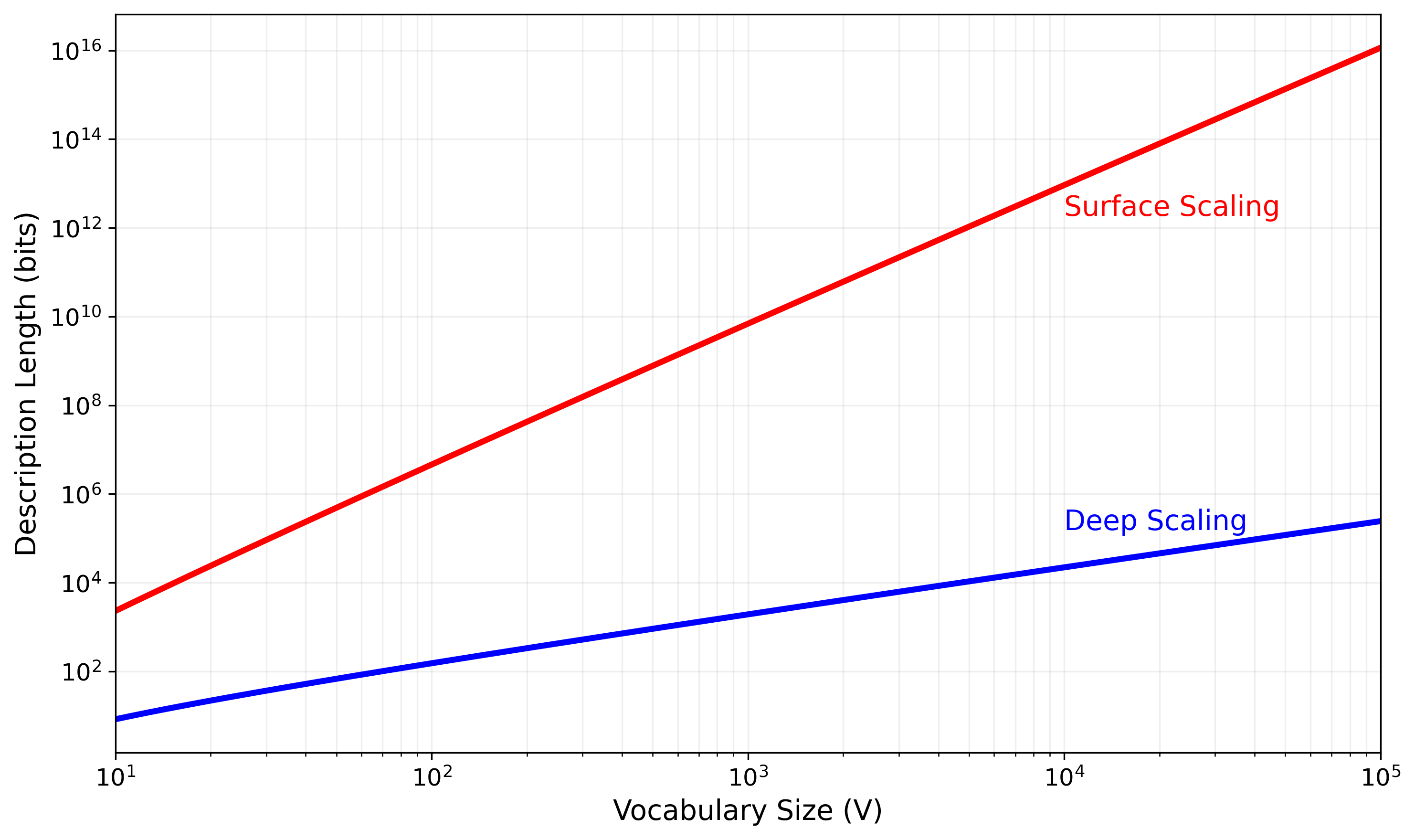Figure 1: Comparison of surface scaling ($\Theta(V^3 \log V)$) vs. deep scaling ($\Theta(V \log \log V)$).

Comparative Scaling and Why Abstraction Wins The difference in scaling is stark:

• Models 0, 1, and 2 have costs tied to the number of sentences or n-grams, which grow polynomially or exponentially with vocabulary size:
  • Model 0 (Rote List): $\Theta(V^3 \log V)$ - explodes with vocabulary
  • Model 1 (N-gram): $\Theta(V^n \log V)$ where $n$ is the n-gram order - explodes even with modest vocabulary increases
  • Model 2 (FSA): $\Theta(V^3 \log V)$ - also explodes with vocabulary
• Model 3’s cost, in contrast, scales primarily as $\Theta(V \log \log V)$, which is dramatically more efficient. Even with a vocabulary of billions of words, this function grows almost linearly with $V$.

This pronounced difference in scaling behavior demonstrates why principled linguistic abstractions (categories and rules) are not just theoretically elegant but practically necessary for efficiently representing and learning something as complex and vast as a natural language. The combinatorial explosion of raw sentences is tamed by factoring out shared properties (categories) and shared structures (rules). Model 3 achieves this factorization, allowing its description length to grow much more gracefully with the scale and complexity of the language. This is the essence of why such structures are fundamental to language’s inherent information efficiency.

The MDL implication is that the most efficient compression of a natural language corpus will necessarily discover and exploit these underlying linguistic abstractions. Categories and rules are not just theoretical constructs; they are information-theoretically optimal ways to encode linguistic complexity.

5. Large Language Models (LLMs) as Efficient Compressors

LLMs are trained to predict the next token, which is mathematically equivalent to minimizing the negative log-likelihood (NLL) of the training corpus. This NLL is a direct measure of the bits needed to encode the corpus using the model’s probability distribution.

$$L(\text{Corpus} \mid \text{Model}) \propto NLL(\text{Corpus} \mid \text{Model})$$

The MDL principle seeks to minimize $L(\text{Model}) + L(\text{Data} \mid \text{Model})$. So, an LLM that better compresses data (lower NLL) by finding a compact model $L(\text{Model})$ makes better predictions.

The drive for predictive accuracy under complexity constraints (e.g., model size) pushes LLMs to discover efficient, principled representations. Evidence suggests LLMs do learn:

• Representations corresponding to syntactic hierarchies (e.g., parse trees and constituent structures). Studies analyzing internal model features, like attention patterns or activations, suggest these are learned even without explicit syntactic supervision.
• Categorical abstractions through word embeddings (words in similar contexts/roles get similar vectors) and more nuanced, context-sensitive representations of word types.
• Systematic generalization to novel combinations (to some extent).

An LLM’s “understanding” can be seen as its success in developing efficient internal representations that mirror language’s abstract principled structure. To achieve high compression and prediction accuracy, they are compelled to discover representations functionally equivalent to the deep principles that make language efficient.

Interestingly, LLMs evolved from simpler neural language models that were essentially implementing Model 1 (n-gram statistics) with neural networks. Classic neural language models like early RNNs were learning to predict the next word based on a fixed window of previous words, similar to n-grams but with dense vector representations. Over time, these models evolved to capture more sophisticated patterns (like those in Model 3) through deeper architectures, attention mechanisms, and transformer designs that could model long-range dependencies and hierarchical structure. This evolution aligns with our scaling analysis: as language models become more powerful, they naturally move toward representations that capture the kind of abstractions present in the principled linguistic model.

This information-theoretic view reveals a profound principle: deeper levels of abstraction enable qualitatively more efficient information packing. This principle extends far beyond language:

1. Information Efficiency Through Abstraction: The exponential efficiency gains we see in Model 3 (principled linguistic structure) compared to surface-level models demonstrate that higher levels of abstraction are not merely convenient organizational tools—they are information-theoretically optimal compression strategies.

2. Hierarchical Compression: By factoring information into layers of abstraction (lexical categories, syntactic rules), we achieve compression rates that are qualitatively superior to flat, surface-level encodings. Each layer of abstraction compounds the efficiency gains.

3. Emergence of Structure: The dramatic scaling advantage of structured representations suggests that any sufficiently powerful learning system under information constraints will naturally discover and exploit these abstractions. This explains why LLMs, despite not being explicitly designed with linguistic theory, appear to develop internal representations that capture deep linguistic regularities.

The fundamental insight is that the universe of possible utterances is vastly more efficiently represented through a hierarchical system of abstractions than through any surface-level statistical approach. This provides a compelling information-theoretic explanation for why our brains might have evolved to process language using hierarchical, structured representations but because it is fundamentally the most efficient way to encode and process the complexities of natural language.

This convergence of information theory, linguistics, and machine learning suggests that the drive toward deeper levels of abstraction is not just a human cognitive bias but a fundamental principle of efficient information processing. As our AI systems grow more sophisticated, we should expect them to discover and leverage increasingly abstract representations—not because we programmed them to do so, but because deeper abstraction is the path to greater information efficiency.