Home / Quantum Gravity / Entropy, action and dynamics

Horizon counts: which weights give the area law

Status

Proved for Poisson sprinklings: expected counts, linear order in uniform curvature of a conformally static family. The necessity of the zeros and the exclusion of non-negative weights (finitely many, or an exponentially decaying kernel) hold for 3 ≤ d ≤ 12, using the positivity of response coefficients computed in exact arithmetic. A finite-curvature integration checks the expansion.

Excludes

Under the stated hypotheses (Poisson sprinkling, expected count, linear order in uniform curvature of the conformally static family, 3 ≤ d ≤ 12): entropy functionals that give each horizon molecule a non-negative amount depending only on its type, with finitely many types or an exponentially decaying kernel, and reproduce the Einstein equation with the area-law Newton constant at every ball size.

Revised

29 October 2026

Which weightings of causal-set horizon molecules make the expected count respond to curvature like the horizon area, at every size of the region, and can such a weighting be non-negative? A horizon molecule is a pair of elements that straddle a horizon just below a spacelike slice, and its type $m$ is the number of further elements in the causal future of the lower element, below the slice. We take a Poisson sprinkling in dimension $d\ge3$, a geodesic ball in the slice, uniform curvature at linear order in a conformally static family of backgrounds, and weights $w_m$ that depend on $m$ only. The response is that of the area if the polynomial $Q(\alpha)=\sum_mw_m(\alpha)_m/m!$ (equation (2); $(\alpha)_m=\alpha(\alpha+1)\cdots(\alpha+m-1)$) is nonzero at $\alpha_A=1+2/d$ and vanishes at the $d$ points $\alpha_A+j/d$, $j=1,\dots,d$ (Theorem 2). For $3\le d\le12$ these zeros are also necessary (Theorem 2(b)), and no non-negative weighting has them, whether it has finitely many nonzero weights or an exponentially decaying kernel (Theorem 3); both use the computed Proposition 2.

The weighting of lowest degree with these zeros is unique up to normalisation, has integer weights that alternate in sign, and in four dimensions is $(210,-791,1268,-928,256)$. A non-negative weighting gives, in the model of section 4, a Newton constant read off from the response of the count to curvature that is strictly smaller than the one set by its own flat-space area law. The Einstein form of the response and the equality of the two Newton constants follow from the zeros alone (Proposition 3), so they do not select among weightings that have them. The mean of the signed count equals the mean of a combination of non-negative counts of thinned sprinklings (Proposition 4), thinning acts on the Mellin symbol by a rescaling (Proposition 5), and no functional of finite marked posets is exactly homogeneous of the area degree under thinning (Proposition 6). All statements concern expected counts.

Barton, Counsell, Dowker, Gould, Jubb and Taylor [Barton et al.] define horizon molecules following the links that Dou and Sorkin [Dou–Sorkin] counted as horizon entropy. They argue, under stated assumptions, that the expected number of links across the horizon tends to a constant times the area of the cross-section as the discreteness length goes to zero, with a leading term local to the cross-section. Machet and Wang [Machet–Wang] argue that a version of the molecule defined by a null hypersurface through the horizon does not give an entropy local to the intersection in a curved spacetime. The molecules below are defined by a spacelike slice, as in [Barton et al.]. Jacobson [Jacobson] derives the Einstein equation from the stationarity of the entropy of small geodesic balls at fixed volume, assuming an area-law entropy, and section 4 applies this to the count. Signed combinations of layer counts with prescribed Mellin zeros define the causal-set d’Alembertian and action [BD] [Dowker–Glaser] [Glaser] [ASS].

Exactness at every order in the gradients of the curvature is the subject of heavy-tailed horizon-count kernels. That page shows, under a hypothesis (H) on the gradient expansion, that a kernel exact at every gradient order and integrable near zero cannot decay at least as fast as the exponential of a fixed multiple of the square root of the linear size of the future region, and that it changes sign infinitely often.

1. Causal sets, sprinklings and horizon molecules

A causal set is a locally finite partially ordered set, read as a discretisation of a Lorentzian manifold in which the order is the causal relation and the number of elements in a region is its volume. A Poisson sprinkling of density $\rho$ into a $d$-dimensional spacetime is a Poisson point process with intensity $\rho$ times the volume measure, ordered by the causal relation $\prec$; its law is invariant under the isometries of Minkowski space. The discreteness length is $\ell_\rho=\rho^{-1/d}$. We set $\rho=1$ except where the density matters, so that lengths are in units of $\ell_\rho$, and $\ell$ denotes the radius of a ball in these units. Two properties of the Poisson process are used throughout. The number of points in a region of volume $V$ is Poisson distributed with mean $\rho V$. The multivariate Mecke equation [Last] says that for a non-negative function $f$ of $k$ points and the process,

$$\mathbb E\sum_{(x_1,\dots,x_k)}f(x_1,\dots,x_k;\eta)=\rho^k\int\mathbb E\,f(x_1,\dots,x_k;\eta+\delta_{x_1}+\dots+\delta_{x_k})\,dx_1\cdots dx_k,$$

where the sum runs over $k$-tuples of distinct points of the process $\eta$: the expectation of a sum over tuples is the integral over their positions of the expectation with the points of the tuple added to the process.

Let $d\ge3$ and $n=d-1$. Let $\Sigma$ be a spacelike slice, $B\subset\Sigma$ a geodesic ball and $o$ the top tip of its domain of dependence. The horizon is the part of $\partial I^-(o)$ below $\Sigma$. It meets $\Sigma$ in $\partial B$, and as one goes to the past its generators move away from $B$, so it has no caustic below $\Sigma$. Write $P=I^-(o)\cap I^-(\Sigma)$ for the region inside the horizon (figure 1).

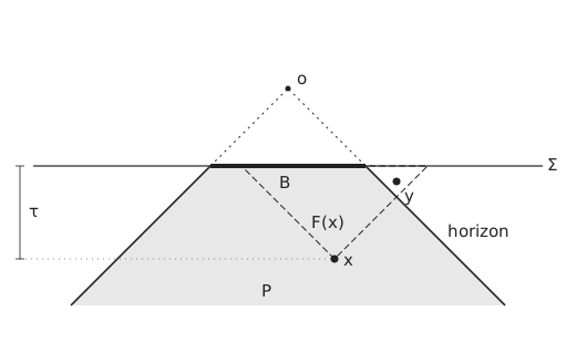
Figure 1. Time runs upward. The horizon leaves $\partial B$ and spreads outward into the past; $P$ is the shaded region below $\Sigma$. The dashed triangle is the part of the future of $x$ that lies below $\Sigma$. The pair $x\prec y$ is a horizon molecule.

For an element $x\in P$ let $F(x)$ be the set of elements in the causal future of $x$ and the past of $\Sigma$. A horizon molecule is a pair $x\prec y$ with $x\in P$ and $y\in F(x)\setminus P$; its type is $m=\lvert F(x)\rvert-1$, the number of elements of $F(x)$ other than $y$, wherever they lie. A molecule of type $0$ is a link $x\prec y$ across the horizon, the molecule of [Barton et al.]. Given real weights $w_0,w_1,\dots,w_K$, the weighted count $H_w$ is the sum of $w_m$ over all molecules, and $H_m$ is the number of molecules of type $m$.

Let $V(x)$ be the volume of $J^+(x)\cap I^-(\Sigma)$ and $V_{\rm out}(x)$ the volume of its part outside $P$. Given $x$ and $y$, the remaining elements of $F(x)$ form a Poisson process of mean $V(x)$, so the probability that there are $m$ of them is $V^me^{-V}/m!$. The Mecke equation with $k=2$ gives

$$\langle H_w\rangle=\int_P dV_x\;V_{\rm out}(x)\,\phi\big(V(x)\big),\qquad \phi(v)=e^{-v}\sum_{m}w_m\frac{v^m}{m!}. \tag{1}$$

The weights enter only through the kernel $\phi$. Its Mellin transform defines the Mellin symbol $Q$ of the weighting,

$$\Gamma(\alpha)\,Q(\alpha)=\int_0^\infty\phi(v)\,v^{\alpha-1}\,dv,\qquad Q(\alpha)=\sum_m w_m\frac{(\alpha)_m}{m!}, \tag{2}$$

where $(\alpha)_m=\alpha(\alpha+1)\cdots(\alpha+m-1)$; the second form follows from $\int_0^\infty v^{m+\alpha-1}e^{-v}dv=\Gamma(\alpha)(\alpha)_m$. A weighting with $w_m=0$ for $m>K$ has a polynomial symbol of degree $K$, and $w\mapsto Q$ is a linear bijection onto polynomials of degree at most $K$, because $(\alpha)_m/m!$ has degree exactly $m$. The weights are recovered from the values of $Q$ at the non-positive integers, using $(-j)_m/m!=(-1)^m\binom jm$ and binomial inversion:

$$w_m=\sum_{j=0}^{m}(-1)^j\binom mj\,Q(-j). \tag{3}$$

The type-0 count has $Q\equiv1$. Section 2 shows that weighting by type multiplies each power of the density in the expected count by the value of $Q$ at a matching exponent; this is why $Q$ is the quantity to prescribe.

2. The mean count in a conformally static background

Let the spacetime be

$$g=W(t)^{2/d}\big(-dt^2+\gamma_A\big),$$

with $\gamma_A$ the round metric on the $n$-sphere of radius $A$ ($A=\infty$ gives flat space) and $W(0)=1$. The power $2/d$ makes the volume element $W\,dt\,dV_\gamma$. Take $\Sigma=\{t=0\}$ and $B$ the geodesic ball of radius $r_0$ about a pole. Write $\omega$ for the volume of the unit $n$-ball, ${\rm cap}(r)$ for the $\gamma_A$-volume of a geodesic ball of radius $\min(r,\pi A)$, and $\ell$ for the radius of the flat ball of the same volume as $B$: ${\rm cap}(r_0)=\omega\ell^n$. The case $W=1$ is the Einstein static universe and $W=\cos^{-d}(t/A)$ is de Sitter space of radius $A$ in conformal time; the slice $t=0$ is the same round sphere in both, with vanishing extrinsic curvature.

Lemma 1 (reduction). With $\tau$ the coordinate depth of $x$ below $\Sigma$,

$$\langle H_w\rangle=\int_0^\infty d\tau\,W(-\tau)\,\phi\big(V(\tau)\big)\,U(\tau), \tag{4}$$ $$U(\tau)=\int_0^\tau ds\,W(s-\tau)\,{\rm cap}(s)\big[{\rm cap}(r_0+\tau)-{\rm cap}(r_0+\tau-s)\big],\qquad V(\tau)=\int_0^\tau ds\,W(s-\tau)\,{\rm cap}(s).$$

Proof. Conformal factors leave the causal relation unchanged, so $(t_1,a)\prec(t_2,b)$ exactly when the $\gamma_A$-distance from $a$ to $b$ is at most $t_2-t_1$. The tip $o$ is at time $r_0$ above the pole, so $P$ at time $-\tau$ is the cap $C_1$ of radius $r_0+\tau$ about the pole, and $V(x)=V(\tau)$ depends only on the depth. An element $y$ at time $s-\tau$ and position $b$ lies in $F(x)$ for $x=(-\tau,a)$ when $b$ is in the cap of radius $s$ about $a$, and lies outside $P$ when $b$ is outside the cap $C_2$ of radius $r_0+\tau-s$ about the pole. Integrating over $a\in C_1$, the volume of positions $b$ in the cap of radius $s$ gives $\mathrm{cap}(s)\,\mathrm{cap}(r_0+\tau)$. The part with $b\in C_2$ is computed by exchanging the roles of $a$ and $b$: for $b\in C_2$ the cap of radius $s$ about $b$ lies inside $C_1$ by the triangle inequality, so it contributes $\mathrm{cap}(s)\,\mathrm{cap}(r_0+\tau-s)$. The volume elements are $W(-\tau)d\tau\,dV_\gamma$ for $x$ and $W(s-\tau)ds\,dV_\gamma$ for $y$.

Equation (4) is exact at any curvature radius $A$, with no wrapping restriction beyond the definition of $\mathrm{cap}$. For de Sitter space the conformal time is restricted to $\lvert t\rvert<\pi A/2$, so the $\tau$-integral ends at $\pi A/2$; since $\phi$ is exponentially small at the volumes reached there, the expansion in $\varepsilon$ below is not affected.

Substituting $v=\omega\tau^d/d$ turns every $\tau$-integral that occurs below into a value of the symbol.

Lemma 2 (moment rule). Let $b=(\sigma+1)/d$ for a real $\sigma\ge0$ and let $r\ge0$ be an integer with $b>r$. Then

$$\int_0^\infty\tau^\sigma\,\phi^{(r)}\!\Big(\frac{\omega\tau^d}{d}\Big)d\tau=(-1)^r\,\frac1d\Big(\frac d\omega\Big)^{b}\,\Gamma(b)\,Q(b-r). \tag{5}$$

Proof. The substitution gives $\frac1d(d/\omega)^b\int_0^\infty v^{b-1}\phi^{(r)}(v)\,dv$. Integrating by parts $r$ times, the boundary terms vanish because $b-j>0$ for $j=1,\dots,r$, and $\int v^{b-1}\phi^{(r)}=(-1)^r(b-1)\cdots(b-r)\int v^{b-r-1}\phi=(-1)^r\Gamma(b)Q(b-r)$ by (2).

It remains to find which value of $Q$ multiplies which term. Expand (4) in the curvature: $\varepsilon=A^{-2}$ and the Taylor coefficients $W_k$ of $W$ (section 3). Every term of the expansion has the form $c\,\ell^e\,\tau^\sigma\,\phi^{(r)}(\omega\tau^d/d)$ with $r\ge0$ derivatives of $\phi$, which come from expanding $\phi(V)$ about the flat volume $V_0=\omega\tau^d/d$ in the corrections to $V$, multiplied by a monomial in $\varepsilon$ and the $W_k$ of length dimension $-\mu$: $\varepsilon^\nu$ has $\mu=2\nu$ and $W_k$ has $\mu=k$. To count powers of length, give $\tau$, $s$, $\ell$ and $A$ dimension $1$ and volumes dimension $d$. Then $U$ has dimension $2n+1=2d-1$ and (4) has dimension $2d$, and $\phi^{(r)}(V)$ has dimension $-rd$. Every term of the expansion has the dimension of (4), so $e+\sigma+1-rd-\mu=2d$, where the $1$ comes from $d\tau$. By (5) the term is multiplied by $Q(b-r)$ with $b=(\sigma+1)/d$, that is, by $Q(\beta)$ with

$$\beta=2-\frac{e-\mu}{d}. \tag{6}$$

In terms of the density the term is proportional to $\rho^{2-\beta}$: a weighting multiplies each power of the density by the value of $Q$ at the matching exponent, and a weighting whose symbol vanishes at all exponents but one keeps a single term of the density expansion. Two terms of the Einstein static universe in $d=4$ show the bookkeeping. The flat count contains the term $3I_1\omega^2\ell^2\tau^5$ of $U$ with $I_1=1/5$ (section 3), so $e=2$, $\sigma=5$, $r=0$, $\mu=0$ and $\beta=2-2/4=3/2$; this is the area exponent $\alpha_A=1+2/d$, and $e+\sigma+1=8=2d$. At first order in $\varepsilon$, the volume is $V=V_0-\omega\varepsilon\tau^6/30$, from the cap volume ${\rm cap}(s)=\omega s^3(1-\varepsilon s^2/5)$, and the flat term of $U$ at order $\ell^0$ is $(17/70)\omega^2\tau^7$, the term $k=3$ of the sum in section 3 with $I_3=17/70$. Their product with $\phi'(V_0)$ is $-(17\omega^3/2100)\,\varepsilon\,\tau^{13}\phi'(V_0)$, with $e=0$, $\sigma=13$, $r=1$, $\mu=2$, and $e+\sigma+1=14=8+2+4$. By (5) it is multiplied by $Q(7/2-1)=Q(5/2)$, in agreement with (6).

3. The flat count and the curvature response

In flat space $W=1$, ${\rm cap}(r)=\omega r^n$ and $V=\omega\tau^d/d$. Expanding the bracket in (4) binomially in $\ell$, the term of order $\ell^n$ cancels and

$$U(\tau)=\omega^2\sum_{k=1}^{n}\binom nkI_k\,\ell^{\,n-k}\tau^{d+k},\qquad I_k=\int_0^1\zeta^n\big[1-(1-\zeta)^k\big]d\zeta=\frac1d-\frac{n!\,k!}{(n+k+1)!}.$$

Proposition 1 (flat count). For a flat ball of radius $\ell$,

$$\langle H_w\rangle=\sum_{k=1}^{n}\binom nkI_k\,\frac{\omega^2}{d}\Big(\frac d\omega\Big)^{\beta_k}\Gamma(\beta_k)\,Q(\beta_k)\,\ell^{\,n-k},\qquad\beta_k=\frac{d+1+k}{d}. \tag{7}$$

There is no term proportional to $\ell^n$, the volume of $B$. The leading term is $Q(\alpha_A)\,a_d\,\lvert\partial B\rvert$ with $\lvert\partial B\rvert=n\omega\ell^{n-1}$ and

$$a_d=\frac{\omega}{d(d+1)}\Big(\frac d\omega\Big)^{\alpha_A}\Gamma(\alpha_A),\qquad\alpha_A=\frac{d+2}{d}. \tag{8}$$

The proof is the computation above followed by (5) with $r=0$, and $I_1=1/(d+1)$ gives (8). The exponents present are $\alpha_A+j/d$ for $0\le j\le d-2$.

Equation (8) gives $a_3=0.218853$, $a_4=\sqrt3/10$, $a_5=0.148656$, $a_6=0.133258$, $a_7=0.122656$, $a_8=0.114883$, and the values for $d=3$ and $4$ are those of [Barton et al.]. In four dimensions

$$\langle H_w\rangle=\frac{2\sqrt3\,\pi}{5}\,Q(\tfrac32)\,\ell^2+\frac{7\cdot3^{3/4}\pi^{1/4}\Gamma(\frac34)}{10}\,Q(\tfrac74)\,\ell+\frac{34}{35}\,Q(2). \tag{9}$$

For the type-0 count this is $2.17656\,\ell^2+2.60322\,\ell+0.97143$.

The response to curvature

In curved space we hold the volume of $B$ fixed at $\omega\ell^n$, so that $\ell$ labels its size, and expand in $\varepsilon=A^{-2}$ and in the Taylor coefficients of $W(t)=1+\sum_{k\ge1}W_kt^k$. The part of the expected count that sits at the area exponent is the exact area of $\partial B$.

Theorem 1 (area exponent). Expand $\langle H_w\rangle$ of (4) as a formal power series in $\varepsilon$ and the $W_k$, with $B$ of fixed volume $\omega\ell^n$.

(a) Every coefficient is a polynomial in $\ell$, and each monomial $\ell^e$ multiplies $Q(\beta)$ with $\beta$ given by (6). A term whose curvature factor has dimension $\mu$ has $\beta=\alpha_A+j/d$ with an integer $j$ satisfying $0\le j\le d-2+\mu$.

(b) Collecting the terms with $\beta=\alpha_A$ over all orders gives exactly $a_d\,Q(\alpha_A)$ times the area of $\partial B$. Every other term has $j\ge1$.

The variable $\ell$ enters (4) only through $r_0$ inside the bracket of $U$. At each order of the curvature expansion the highest power of $\ell$ therefore comes from the first derivative ${\rm cap}'(r_0)$, which is the area of $\partial B$, with every other factor at its flat value; that term sits at the area exponent.

Proof. The cap volume is ${\rm cap}(r)=\sum_\nu\omega_\nu\varepsilon^\nu r^{n+2\nu}$ with $\omega_0=\omega$, and the fixed-volume condition gives $r_0=\ell\,\psi(\varepsilon\ell^2)$ for a power series $\psi$ with $\psi(0)=1$. Expand the bracket of $U$ as $\sum_{i\ge1}{\rm cap}^{(i)}(r_0)\,[\tau^i-(\tau-s)^i]/i!$. The part of order $\varepsilon^\nu$ of ${\rm cap}^{(i)}(r_0)$ is a constant times $\ell^{\,n+2\nu-i}$, since each power of $\varepsilon$ that comes through $r_0$ or the cap series carries $\ell^2$. No other factor of (4), including the expansion of $\phi(V)$ about $\omega\tau^d/d$ and the factors $W$, depends on $\ell$, and their $\tau$- and $s$-integrals are finite polynomials. So each coefficient is a polynomial in $\ell$, with $e\ge0$. In a term of order $\varepsilon^\nu$ with total curvature dimension $\mu=2\nu+\mu'$, where $\mu'$ comes from the $W_k$, the power of $\ell$ is at most $n-1+2\nu$, with equality only if $i=1$, the other factors of that term contain no $\varepsilon$, and $\mu'=0$ (no $W_k$ and no volume correction $V-V_0$, which carries one). Then (6) gives $\beta\ge 2-\frac{n-1+2\nu-2\nu-\mu'}{d}=\alpha_A+\mu'/d$, with equality exactly in the case just described. That term is $[{\rm cap}'(r_0)]_\nu\int_0^\infty d\tau\,\phi(\omega\tau^d/d)\int_0^\tau ds\,\omega s^{n}\,s$, which by the flat computation equals $a_dQ(\alpha_A)[{\rm cap}'(r_0)]_\nu$, and ${\rm cap}'(r_0)=\lvert\partial B\rvert$ is the exact area of the boundary of the geodesic ball. Since $e$ and $\mu$ are integers, $\beta=\alpha_A+j/d$ with $j=d-2-e+\mu$, and $e\ge0$ gives $j\le d-2+\mu$.

At linear order in the curvature and for curvature that is uniform over the ball, two backgrounds suffice. Write $u$ for the unit normal of $\Sigma$. The static universe ($W=1$) has scalar curvature of the slice $R^\Sigma=n(n-1)/A^2$ and $R_{uu}=0$; de Sitter space in conformal time has the same slice and $R_{uu}=-n/A^2$. We define the response at fixed volume by

$$\delta\langle H_w\rangle\big|_V=-h_\Sigma(\ell)\,R^\Sigma-h_0(\ell)\,R_{uu}, \tag{10}$$

where $h_\Sigma$ and $h_0$ are determined by the two backgrounds. We assume that for any perturbation whose curvature is uniform over the ball and whose slice has vanishing extrinsic curvature at the centre, the linear response is a rotation-invariant linear function of the Riemann tensor at the centre. The only such scalars are $R^\Sigma$ and $R_{uu}$, because the Weyl tensor enters through its electric part, which is traceless and averages to zero over directions. This assumption is used only to say that (10) describes all uniform curvatures; all statements about $h_\Sigma$ and $h_0$ below are about the two backgrounds.

A geodesic sphere of radius $r$ has area $n\omega r^{n-1}\big(1-R^\Sigma r^2/(6n)\big)$ and encloses volume $\omega r^n\big(1-R^\Sigma r^2/(6(n+2))\big)$ to first order; the first is the derivative of the second with respect to $r$. Eliminating $r$ at fixed volume, $r=\ell\big(1+R^\Sigma\ell^2/(6n(n+2))\big)$, gives the area $n\omega\ell^{n-1}\big(1-R^\Sigma\ell^2/(2n(n+2))\big)$ and the area deficit used by Jacobson [Jacobson],

$$\delta\lvert\partial B\rvert\big|_V=-c_d\,\ell^dR^\Sigma,\qquad c_d=\frac{\omega}{2(d+1)}\quad(c_4=2\pi/15). \tag{11}$$

By Theorem 1 the part of $h_\Sigma$ at the area exponent is $a_dQ(\alpha_A)c_d\ell^d$. The coefficient $h_0$ has no part at the area exponent, because the two backgrounds have the same slice and the same ball.

The remaining coefficients follow from (4) by expanding to first order in $\varepsilon$ with $W=1+\tfrac d2\varepsilon t^2$ for de Sitter space: each monomial in $\tau$ is integrated with (5), and a term $\phi'$ from the change of $V$ gives $-\Gamma(b)Q(b-1)$. We carried this out in exact arithmetic for $d=3,\dots,12$. The expansion is evaluated term by term without a general proof, so we test it in $d=4$ with $\ell=1$: integrating (4) numerically with the exact caps and $W=\cos^{-4}(t/A)$ at finite $A$ and extrapolating in $A^{-2}$ reproduces the first-order coefficients of the expansion, $-4.24641$ (static) and $8.0812$ (de Sitter), to a relative accuracy of $10^{-6}$.

In four dimensions, with each entry multiplied by $Q$ at the exponent in the first column, the result is

exponent $\alpha$	flat count	$h_\Sigma$	$h_0$
$3/2$	$\frac{2\sqrt3\pi}{5}\ell^2$	$\frac{\sqrt3\pi}{75}\ell^4$	$0$
$7/4$	$\frac{7\cdot3^{3/4}\pi^{1/4}\Gamma(3/4)}{10}\ell$	$\frac{7\cdot3^{3/4}\pi^{1/4}\Gamma(3/4)}{100}\ell^3$	$0$
$2$	$\frac{34}{35}$	$\frac{48}{175}\ell^2$	$\frac{256}{175}\ell^2$
$9/4$		$\frac{31\cdot3^{1/4}\Gamma(1/4)}{1120\,\pi^{1/4}}\ell$	$\frac{37\cdot3^{1/4}\Gamma(1/4)}{70\,\pi^{1/4}}\ell$
$5/2$		$\frac{\sqrt3}{1260}$	$\frac{547\sqrt3}{1260}$

and in three dimensions the flat count is $\frac{3^{2/3}\pi^{1/3}\Gamma(2/3)}{3}Q(\tfrac53)\ell+\frac9{10}Q(2)$, with $h_\Sigma=\frac{3^{2/3}\pi^{1/3}\Gamma(2/3)}{48}Q(\tfrac53)\ell^3+\frac9{40}Q(2)\ell^2+\frac{3^{1/3}\Gamma(1/3)}{20\pi^{1/3}}Q(\tfrac73)\ell+\frac{3^{2/3}\Gamma(2/3)}{210\pi^{2/3}}Q(\tfrac83)$ and $h_0=\frac{5\cdot3^{1/3}\Gamma(1/3)}{12\pi^{1/3}}Q(\tfrac73)\ell+\frac{64\cdot3^{2/3}\Gamma(2/3)}{105\pi^{2/3}}Q(\tfrac83)$. The five-dimensional coefficients, to six figures, are in the table below.

exponent $\alpha$	flat count	$h_\Sigma$	$h_0$
$7/5$	$2.93435\,\ell^3$	$0.0611322\,\ell^5$	$0$
$8/5$	$5.07907\,\ell^2$	$0.282170\,\ell^4$	$0$
$9/5$	$3.64942\,\ell$	$0.435442\,\ell^3$	$1.83853\,\ell^3$
$2$	$0.992063$	$0.302343\,\ell^2$	$3.38010\,\ell^2$
$11/5$		$0.0808902\,\ell$	$2.54882\,\ell$
$12/5$		$0.000321766$	$0.721238$

Proposition 2 (structure of the response, $3\le d\le12$, computed). Let $3\le d\le12$. With exponents $\alpha_A+j/d$ and each coefficient multiplying $Q$ at its exponent, the flat count has nonzero coefficients exactly for $0\le j\le d-2$, $h_\Sigma$ for $0\le j\le d$, and $h_0$ for $2\le j\le d$, and every one of these coefficients is positive. The coefficient of $h_\Sigma$ at $j=0$ is $a_dc_d\ell^d$.

The statement is the outcome of the expansion described above, carried out in exact rational arithmetic for each $d$ from $3$ to $12$; the tables show $d=3,4,5$. We have no closed form for the coefficients as functions of $d$ and $j$, so $d\le12$ is the range computed. Theorem 1 already gives the upper limits $j\le d-2$ for the flat count and $j\le d$ at first order, and the sentence after (11) gives the absence of a term at $j=0$ in $h_0$. Proposition 2 adds that $h_0$ has no term at $j=1$, that no coefficient inside the stated ranges vanishes, and that all are positive.

4. Entanglement equilibrium and the Newton constant

We model the use of the count as in Jacobson’s argument [Jacobson], with a causal-set count in place of the entanglement entropy of short-distance degrees of freedom. The entropy of the region is $s_0\langle H_w\rangle$ for a constant $s_0$. In flat space this defines the Newton constant $G$ through $S=\lvert\partial B\rvert/4G$ at leading order, so $1/(4G)=s_0Q(\alpha_A)a_d\,\rho^{(d-2)/d}$. Entanglement equilibrium holds: at fixed volume the change of the short-distance entropy balances the change of the matter entropy. In Jacobson’s argument the entropy of a small ball is the sum of a short-distance part and the entropy of the matter fields, and the vacuum is taken to be stationary under variations at fixed volume, so the two variations cancel. Imposed for every unit timelike $u$, this balance is equivalent to the Einstein equation with coupling $G_N$ if the short-distance entropy varies by $\delta\lvert\partial B\rvert_V/4G_N$. On a slice with vanishing extrinsic curvature the Gauss equation gives $R^\Sigma=2G_{uu}$, so by (11) $\delta\lvert\partial B\rvert_V=-2c_d\ell^dG_{uu}$. The count gives the variation $-s_0h_\Sigma R^\Sigma-s_0h_0R_{uu}$ by (10), and $s_0=1/(4GQ(\alpha_A)a_d)$ by the definition of $G$. Matching the two variations with $G_N=G$ requires $h_0=0$ and $h_\Sigma=Q(\alpha_A)a_dc_d\ell^dG/G_N$, so the count reproduces the linearised Einstein equation with $G_N=G$ at size $\ell$ exactly when

(i) $h_0(\ell)=0$, and (ii) $h_\Sigma(\ell)=Q(\alpha_A)\,a_d\,c_d\,\ell^d$.

If (i) fails, the response depends on $R_{uu}$ separately and the equation is not Einstein’s. For matter with $R_{uu}=\lambda R^\Sigma$ we define $G_N/G=Q(\alpha_A)a_dc_d\ell^d/(h_\Sigma+\lambda h_0)$. In four dimensions, with energy density $\varrho$ and isotropic pressure $\varpi$, the Einstein equation $R_{ab}=8\pi G_N(T_{ab}-\tfrac12Tg_{ab})$ gives $R^\Sigma=2G_{uu}=16\pi G_N\varrho$ and $R_{uu}=4\pi G_N(\varrho+3\varpi)$, hence $\lambda=(\varrho+3\varpi)/(4\varrho)$: $\lambda=0$ for $\varpi=-\varrho/3$, where only the slice curvature enters, $\lambda=1/4$ for dust and $\lambda=1/2$ for radiation. This is the definition of $G_N/G$ used below. It is a model: only the expected count enters, and fluctuations of the count are ignored.

For the type-0 count ($Q\equiv1$), the table of section 3 gives in four dimensions and for $\lambda=0$

$$\frac{G_N}{G}=\frac{1}{1+3.588/\ell+3.781/\ell^2+1.367/\ell^3+0.019/\ell^4}\qquad(\text{type-0 weights},\ \ell\text{ in units of }\ell_\rho).$$

Both conditions therefore hold up to relative corrections of order $\ell_\rho/\ell$ for large balls, and they fail for balls a few discreteness lengths across. To see the size of the effect for a population of balls, take those spanned by links. A causal diamond of half-height $\ell$ has volume $2\pi\ell^4/3$ in four dimensions, and a related pair is a link when its diamond is empty. For a fixed upper element, the elements of its past at proper time $2\ell$ lie on a hyperboloid, and the number of related pairs with half-height in $d\ell$ grows as $\ell^3d\ell$. The half-heights of links are therefore distributed as $\ell^3e^{-2\pi\ell^4/3}$. Averaging the numerator and the denominator of $G_N/G$ over this distribution, the type-0 count gives $G_N/G=0.0832$, $0.0292$ and $0.0177$ for $\lambda=0$, $1/4$ and $1/2$.

5. Weights that remove the non-area exponents

The terms of the response other than the one at the area exponent are the obstruction to conditions (i) and (ii). If $Q$ vanishes at their exponents, they drop out, whatever the weights are elsewhere.

Proposition 3 (removal of non-area exponents). Let $\phi$ be the kernel (1) of a finite weighting and let $Q(\alpha_A)\neq0$. Suppose $Q$ vanishes at every exponent $\alpha_A+j/d$ with $j\ge1$ that occurs in the flat count, in $h_\Sigma$ or in $h_0$. Then the flat count is $Q(\alpha_A)a_d\lvert\partial B\rvert$, the response is $Q(\alpha_A)a_d\,\delta\lvert\partial B\rvert_V$, so that $h_0\equiv0$ and $h_\Sigma=Q(\alpha_A)a_dc_d\ell^d$, and $G_N/G\equiv1$ for every $\lambda$.

Proof. By Theorem 1(b) the terms at the area exponent sum to $a_dQ(\alpha_A)$ times the exact area of $\partial B$, and every other term carries $Q$ at one of the zeros. The static universe and de Sitter space have the same slice and the same ball, so the area-exponent part of the first-order coefficient is the same in both, and equals $a_dQ(\alpha_A)\,\delta\lvert\partial B\rvert_V$. Hence $h_0$, which is the difference of the two, has no surviving part, and $h_\Sigma=a_dQ(\alpha_A)c_d\ell^d$ by (11).

The Einstein form and $G_N=G$ therefore hold for every weighting that removes the non-area exponents, and cannot be used to select among such weightings. They can fail only for a weighting that keeps a non-area exponent. Theorem 1(a) bounds the exponents that can occur, and the next theorem turns this into a finite list of zeros.

Theorem 2 (exact weights). Let $d\ge3$ and let $w$ be a finite weighting with $Q(\alpha_A)\neq0$.

(a) If $Q(\alpha_A+j/d)=0$ for $j=1,\dots,d$, then for every $\ell>0$ the flat count equals $Q(\alpha_A)a_d\lvert\partial B\rvert$ and conditions (i) and (ii) hold.

(b) Let $3\le d\le12$. If condition (ii) holds for all $\ell>0$, then $Q(\alpha_A+j/d)=0$ for $j=1,\dots,d$. This part uses Proposition 2.

(c) A weighting with these zeros has $w_m\neq0$ for some $m\ge d$. Among weightings with $w_m=0$ for $m>d$ it is unique up to normalisation, and

$$Q_d(\alpha)=\binom{2d+2-d\alpha}{d},\qquad w_m=\sum_{j=0}^{m}(-1)^j\binom mj\binom{2d+2+dj}{d}. \tag{12}$$

Proof. (a) By Theorem 1(a) the exponents other than $\alpha_A$ that occur in the flat count ($\mu=0$) and at first order in the curvature ($\mu=2$) are among $\alpha_A+j/d$ with $1\le j\le d$. These are the prescribed zeros, and Proposition 3 gives the claim. (b) By Proposition 2 the function $h_\Sigma-Q(\alpha_A)a_dc_d\ell^d=\sum_{j=1}^dC^\Sigma_jQ(\alpha_A+j/d)\ell^{d-j}$ has all $C^\Sigma_j\neq0$, and the powers $\ell^{d-j}$ are distinct. It vanishes for all $\ell>0$ only if each $Q(\alpha_A+j/d)$ vanishes. (c) A polynomial of degree $N$ with $d$ prescribed zeros that is not identically zero has $N\ge d$, and for $N=d$ it is fixed up to a constant by its zeros. With $z=2d+2-d\alpha$, $\binom zd=z(z-1)\cdots(z-d+1)/d!$ vanishes at $z=0,\dots,d-1$, which are the points $\alpha=\alpha_A+j/d$, $j=d,\dots,1$, and equals $1$ at $z=d$, which is $\alpha=\alpha_A$. The weights follow from (3), since $Q_d(-j)=\binom{2d+2+dj}{d}$.

Part (a) holds in every dimension $d\ge3$ because it needs only the range of $j$ in Theorem 1(a). Part (b) and the exclusion in section 6 need the nonvanishing and the signs of the coefficients, which are computed for $d\le12$. The weights are integers, with $w_0=\binom{2d+2}{d}$ and $w_d=(-d)^d$:

$d$	zeros of $Q_d$	weights $w_0,\dots,w_d$	$a_d$
3	$2,\ \tfrac73,\ \tfrac83$	$56,\ -109,\ 90,\ -27$	$0.218853$
4	$\tfrac74,\ 2,\ \tfrac94,\ \tfrac52$	$210,\ -791,\ 1268,\ -928,\ 256$	$0.173205$
5	$\tfrac85,\ \tfrac95,\ 2,\ \tfrac{11}5,\ \tfrac{12}5$	$792,\ -5396,\ 14750,\ -19500,\ 12500,\ -3125$	$0.148656$
6	$\tfrac32,\dots,\tfrac73$	$3003,\ -35757,\ 155713,\ -328779,\ 365256,\ -206064,\ 46656$	$0.133258$

For $d=7$ and $8$ the weights are

$$(11440,-233717,1556926,-4912103,8384292,-7983325,4000066,-823543)$$

and

$$(43758,-1518517,15075412,-68204640,167489792,-238911488,198377472,-89128960,16777216).$$

For $K>d$ there is a family of dimension $K-d$, and “unique” means unique at minimal degree. For example in $d=4$ with $K=5$ the solutions are the minimal one plus a multiple of $Q_4(\alpha)(\alpha-\tfrac32)$.

A weighting that keeps one of the non-area exponents fails. In four dimensions, keeping $\alpha=2$ with $Q(2)=q\neq0$ and the other three zeros gives $h_0=\tfrac{256}{175}q\,\ell^2\neq0$.

Remark (relation to the causal-set d’Alembertian). Benincasa and Dowker [BD] define, for density $\rho=\ell_\rho^{-4}$ in four dimensions, the operator

$$\Box_{\rm cs}f(x)=\frac{4}{\sqrt6\,\ell_\rho^{2}}\Big[-f(x)+\sum_{i=1}^{4}w_{i-1}\sum_{y\in L_i(x)}f(y)\Big],\qquad(w_0,w_1,w_2,w_3)=(1,-9,16,-8),$$

where $L_i(x)$ is the set of elements $y\prec x$ with $i-1$ elements between $y$ and $x$. The mean of $\Box_{\rm cs}f$ tends to the flat d’Alembertian of $f$ as $\ell_\rho\to0$; in the signature $(-,+,+,+)$ of this page the d’Alembertian is $-\partial_t^2+\nabla^2$. The coefficients $w_{i-1}$ are the weights of a kernel of the form (1), with symbol $Q_{\rm BD}(\alpha)=-\tfrac43(\alpha-\tfrac12)(\alpha-1)(\alpha-\tfrac32)$ by (2), so the zeros are spaced by $2/d$. The action of the same paper, $N-N_1+9N_2-16N_3+8N_4$ with $N_i$ the number of order intervals of $i+1$ elements, carries the opposite sign on these coefficients, so the symbol of its weights, $\tfrac13(2s-1)(s-1)(2s-3)$, is minus the $Q_{\rm BD}$ printed here; it is the one called $Q_{\rm BD}$ on boundary and corner terms and causal-set counts and dimensionless constants. The zeros of $Q_4$ are $\tfrac74,2,\tfrac94,\tfrac52$, spaced by $1/d$ and all above $\alpha_A=\tfrac32$, and $Q_4(\alpha_A)=1$.

6. No non-negative weighting

Theorem 2 asks $Q$ to vanish at positive points. A non-negative kernel cannot do that.

Theorem 3 (no non-negative weighting). (a) Let $\phi\ge0$ be a measurable function on $(0,\infty)$, not almost everywhere zero, whose Mellin integral $\int\phi\,v^{\alpha-1}dv$ converges at the $\alpha>0$ in question. Then $Q(\alpha)>0$ in (2), and no zero required in Theorem 2 can occur. Non-negative weights $w_m$, not all zero, give such a $\phi$ at $\alpha$ exactly when $\sum_mw_mm^{\alpha-1}<\infty$, in particular when finitely many are nonzero; for $w_m=1$ for all $m$, $\phi\equiv1$ and the integral diverges at every $\alpha$.

(b) Let $3\le d\le12$, and let the weighting be non-negative with finitely many nonzero weights, or non-negative with a smooth kernel that decays exponentially together with its derivatives (the setting in which the expansion of sections 2 and 3 is defined), or a finite positive combination of dilates $\phi(c\,\cdot)$ of such kernels. Then $h_0(\ell)>0$ and $h_\Sigma(\ell)>Q(\alpha_A)a_dc_d\ell^d$ for every $\ell>0$, so that $G_N<G$ for every $\lambda\ge0$, at every ball size, and for every population of sizes with non-negative weight. This part uses Proposition 2.

Proof. (a) is (2): $\Gamma(\alpha)Q(\alpha)=\int\phi\,v^{\alpha-1}dv>0$. (b) The functions $h_0$ and $h_\Sigma-Q(\alpha_A)a_dc_d\ell^d$ are sums of positive coefficients (Proposition 2) times positive values $Q(\alpha_A+j/d)$ by (a), which applies because $\phi$ has finitely many terms or decays exponentially, so that its Mellin integral converges at every $\alpha>0$. A dilate changes $Q$ to $c^{-\alpha}Q$, since $M[\phi(c\,\cdot)](\alpha)=c^{-\alpha}M[\phi](\alpha)$, which keeps the values positive. The ratio $G_N/G$ for a population is the ratio of two averages, and each is bounded by the corresponding bound pointwise.

Part (a) is the sign of an integral. For non-negative infinite weights that satisfy neither the moment condition nor the exponential decay, $h_\Sigma$ and $h_0$ are not defined by the expansion used here, and the theorem makes no statement about them. Part (b) uses Proposition 2, which shows that every non-area term contributes with the same sign. The theorem does not cover substrates with signed correlations, where the expectation (1) is not an integral against a non-negative measure. In the setting of the theorem, an entropy that gives each molecule a positive amount depending on its type yields a weaker gravitational coupling than its own area law at finite density, for $d\le12$ and $\lambda\ge0$. The number of sign changes of the kernel is bounded below by the number of zeros of $Q$.

Lemma 3 (sign changes). Let $\phi$ be continuous on $(0,\infty)$ with finitely many sign changes, and suppose $\int_0^\infty\phi(v)v^{\alpha_k-1}dv=0$, with absolute convergence, for $Z$ distinct real $\alpha_k$. Then $\phi\equiv0$ or $\phi$ changes sign at least $Z$ times.

Proof. Suppose $\phi$ changes sign exactly at $v_1<\dots<v_r$ with $r<Z$. A nonzero combination $\sum_{k=1}^{r+1}c_kv^{\alpha_k-1}$ has at most $r$ positive zeros counted with multiplicity (Descartes’ rule for generalised polynomials), and the $r$ linear conditions that it vanish at the $v_i$ have a nonzero solution. That solution changes sign exactly at the $v_i$, so its product with $\phi$ has one sign, and its integral against $\phi$ is zero by hypothesis, which forces $\phi\equiv0$.

Corollary 1 (alternation). If $w$ is not identically zero, $w_m=0$ for $m>N$ and $Q$ vanishes at $N$ positive points, then $w_0,\dots,w_N$ are all nonzero and strictly alternate in sign. In particular the weights (12) alternate.

Proof. By Lemma 3 the function $\phi=e^{-v}p(v)$, $p(v)=\sum w_mv^m/m!$, changes sign at least $N$ times, so $p$ has at least $N$ positive zeros. By Descartes’ rule its $N+1$ coefficients then have at least $N$ sign changes, which forces all of them to be nonzero with alternating signs.

For $d=4$, $\phi(v)=e^{-v}\big(210-791v+634v^2-\tfrac{464}{3}v^3+\tfrac{32}{3}v^4\big)$ changes sign at $v=0.361$, $1.583$, $4.052$ and $8.504$, and ranges between $-41.8$ and $210$. The area term is the moment $\int\phi\,v^{1/2}dv/\Gamma(\tfrac32)=1$, while $\int\lvert\phi\rvert v^{1/2}dv/\Gamma(\tfrac32)=114.9$: the area term is the net of positive and negative contributions whose total absolute value is $115$ times larger. For the symbols $\binom{N+6-4\alpha}{N}$, which equal $1$ at $\alpha_A$ and vanish at $\alpha_A+j/4$ for $j=1,\dots,N$ ($N=4$ is $Q_4$, and $N=6$ removes the exponents needed at the first gradient order, section 9), the same ratio is $929$, $7.2\times10^3$ and $4.0\times10^5$ for $N=6,8,12$, a factor of about $2.8$ per added zero.

The weights themselves grow at least geometrically. From $Q(-j)=\sum_mw_m(-1)^m\binom jm$ and $\binom jm\le2^j$ one gets $\sum_m\lvert w_m\rvert\ge Q(-j)/2^j$ for every $j\ge0$, and $j=N$ gives $\sum_m\lvert w_m\rvert\ge\binom{5N+6}{N}2^{-N}$, which grows like $6.1^N$. The sums $\sum_m\lvert w_m\rvert$ for the weights of these symbols are $3453$, $1.4\times10^5$, $5.4\times10^6$ and $8.4\times10^9$ for $N=4,6,8,12$. A signed count of this type is a small difference of large terms.

7. The signed count as an extrapolation of positive counts

Let $C_p$ be the type-0 count of the $p$-thinned sprinkling, in which each element is kept independently with probability $p$. It is a positive count.

Proposition 4 (Richardson representation). (i) For every sprinkling $\eta$, $\mathbb E[C_p\mid\eta]=p^2\sum_m(1-p)^mH_m(\eta)$. (ii) Suppose the expected molecule numbers have the form $\langle H_m\rangle=\sum_{j=0}^d\kappa_j\frac{(\alpha_j)_m}{m!}$ with $\alpha_j=\alpha_A+j/d$; by Lemma 2 this is the form of the flat count and of every term of the curvature response at first order, with $\kappa_j$ the coefficient of $Q(\alpha_j)$. Then $\mathbb E\,C_p=\sum_j\kappa_jp^{2-\alpha_j}$. For distinct $p_0,\dots,p_d\in(0,1]$ the system $\sum_i\theta_ip_i^{2-\alpha_j}=\delta_{j0}$, $j=0,\dots,d$, has a unique solution, and

$$\mathbb E\,H_{Q_d}=\sum_{i=0}^d\theta_i\,\mathbb E\,C_{p_i}=\kappa_0.$$

Proof. (i) A pair $x\prec y$ with $x$ inside and $y$ outside survives the thinning with probability $p^2$, and it is a type-0 molecule of the thinned sprinkling exactly when the other $m$ elements of $F(x)$ are all deleted, which has probability $(1-p)^m$ independently of the rest. (ii) The binomial series gives $\sum_m(1-p)^m(\alpha)_m/m!=p^{-\alpha}$, so $\mathbb E\,C_p=p^2\sum_m(1-p)^m\langle H_m\rangle=\sum_j\kappa_jp^{2-\alpha_j}$. The matrix $p_i^{2-\alpha_j}=p_i^{1-2/d}\,(p_i^{-1/d})^j$ is a row-scaled Vandermonde matrix and is nonsingular. Finally $\mathbb E\,H_{Q_d}=\sum_j\kappa_jQ_d(\alpha_j)=\kappa_0$.

The expected signed count therefore equals the expected value of a combination of positive counts of thinned sprinklings: the mean of $H_{Q_d}$ is a Richardson extrapolation of the type-0 count to infinite density at fixed $\ell$, performed at one density by thinning. The coefficients $\theta_i$ cannot all be non-negative, since $\sum_i\theta_ip_i^{2-\alpha_j}=0$ for $j\ge1$ with positive terms $p_i^{2-\alpha_j}$ would force $\theta=0$; this is Theorem 3 seen from the other side.

The identity is about means and does not fix the distribution. Besides $H_{Q_d}(\eta)$ itself, two further random variables have the same mean: the Rao–Blackwellised combination $\sum_i \theta_i\,\mathbb E[C_{p_i}\mid\eta]=\sum_m\tilde w_mH_m(\eta)$ with $\tilde w_m=\sum_i\theta_ip_i^2(1-p_i)^m$, and the combination $\sum_i\theta_iC_{p_i}(\eta_{p_i})$ of independently thinned copies. The count $H_{Q_d}$ and the Rao–Blackwellised combination have weights of both signs: for the weights $w$ of (12) by Corollary 1, and for $\tilde w$ by Theorem 3(a), whose kernel $\sum_i\theta_ip_i^2e^{-p_iv}$ is a finite sum of exponentials and has a finite Mellin integral; its symbol $\sum_i\theta_ip_i^{2-\alpha}$ vanishes at $\alpha_A+j/d$ for $j\ge1$, which Theorem 3(a) excludes for non-negative $\tilde w$. The three variables have different distributions on a given sprinkling, so the sign of the count on one sprinkling depends on which representation of the mean is used, and the mean does not fix it.

8. Thinning

Thinning acts on a weighting through a matrix, and its action on the Mellin symbol is a rescaling. Let $(\Xi_pw)(m)=\sum_{k}\binom mkp^k(1-p)^{m-k}w_k$ be the weights of a molecule of type $m$ after each of its $m$ extra elements is kept independently with probability $p$, so that for a given sprinkling $\mathbb E[H_w(\eta_p)\mid\eta]=p^2\sum_{\text{molecules}}(\Xi_pw)(m)$.

Proposition 5 (thinning duality and sign class). For a finite weighting $w$ and $p\in(0,1]$:

(a) $\sum_m(\Xi_pw)(m)\dfrac{(\alpha)_m}{m!}=p^{-\alpha}Q_w(\alpha)$.

(b) The kernel of $\Xi_pw$ is $\phi_{\Xi_pw}(v)=\phi_w(pv)$.

(c) If $\Xi_pw\ge0$ for some $p\in(0,1]$ then $\phi_w\ge0$ and $Q_w$ has no positive zero. Consequently, if $Q_w$ has a positive zero, as every weighting of Theorem 2 does, then $\Xi_pw$ takes a negative value for every $p\in(0,1]$.

(d) The number of sign changes of the kernel $\phi_{\Xi_pw}$ is independent of $p$, and by Lemma 3 it is at least the number of positive zeros of $Q_w$.

Proof. (a) Write $\binom mk\frac{(\alpha)_m}{m!}=\frac{(\alpha)_k}{k!}\frac{(\alpha+k)_{m-k}}{(m-k)!}$. Summing over $m$ first, $\sum_{j\ge0}\frac{(\alpha+k)_j}{j!}(1-p)^j=p^{-\alpha-k}$, so the sum is $\sum_kw_kp^k\frac{(\alpha)_k}{k!}p^{-\alpha-k}=p^{-\alpha}Q_w(\alpha)$. (b) $e^{-\lambda}\sum_m(\Xi_pw)(m)\lambda^m/m!=e^{-\lambda}e^{(1-p)\lambda}\sum_kw_k(p\lambda)^k/k!=\phi_w(p\lambda)$. (c) If $\Xi_pw\ge0$ the left side of (b) is non-negative, so $\phi_w(pv)\ge0$ for all $v$, hence $\phi_w\ge0$, and Theorem 3(a) applies. (d) follows from (b), since $v\mapsto pv$ is increasing.

By part (a) the thinned weights $p^{\alpha_A}\Xi_pw$, which have infinite support, have symbol $p^{\alpha_A-\alpha}Q_w(\alpha)$: the same zeros and the same value at the area exponent. Proposition 3 holds verbatim for them. Its proof uses Theorem 1, Lemma 2 and the zeros of the symbol, and Theorem 1 and Lemma 2 need only a smooth kernel with exponential decay, which $\phi_w(pv)$ is. The kernel $\phi_w(pv)$ has the same number of sign changes as $\phi_w$. Their counts are related to the thinned sprinkling by $H_{p^{\alpha_A}\Xi_pw}(\eta)=p^{\alpha_A-2}\,\mathbb E[H_w(\eta_p)\mid\eta]$. Thinning the sprinkling and then applying an exact weighting therefore gives, on average, another exact weighting, with the same number of kernel sign changes, and by part (c) never a non-negative one.

The area term of the expected count scales as $\rho^{(d-2)/d}$, so one may ask whether a functional of the sprinkling can be exactly homogeneous of this degree under thinning. For a functional of finite orders it cannot. A marked poset is a pair $(X,D)$ of a finite poset $X$ and a down-set $D\subseteq X$; in a sprinkling $D$ plays the role of the elements inside the horizon, and the $p$-thinning $X_p$ keeps each element of $X$ independently with probability $p$.

Proposition 6 (no exact finite-order homogeneity). Let $F$ be an isomorphism-invariant real function on finite marked posets $(X,D)$ with $F(\emptyset)=0$. If $\mathbb E\,F(X_p)=p^\gamma F(X)$ for all finite $(X,D)$ and all $p\in(0,1]$, then either $\gamma$ is a positive integer, or $F\equiv0$. In particular, for $d\ge2$ the area degree $\gamma=(d-2)/d\in[0,1)$ is not a positive integer, and no nonzero functional of finite marked posets is exactly homogeneous of that degree.

Proof. The sub-poset kept by the thinning is a subset $S\subseteq X$ with probability $p^{\lvert S\rvert}(1-p)^{\lvert X\rvert-\lvert S\rvert}$, so $\mathbb E\,F(X_p)=\sum_{S\subseteq X}p^{\lvert S\rvert}(1-p)^{\lvert X\rvert-\lvert S\rvert}F(S)$ is a polynomial in $p$ that tends to $F(\emptyset)=0$ as $p\to0$. If $\gamma$ is not an integer, $p^\gamma F(X)$ is a polynomial on $(0,1]$ only if $F(X)=0$. If $\gamma$ is a negative integer, $p^\gamma F(X)$ is unbounded as $p\to0$ unless $F(X)=0$, while the polynomial is bounded. If $\gamma=0$, the polynomial equals the constant $F(X)$ and its limit at $p=0$ gives $F(X)=0$.

The proposition concerns exact homogeneity of a functional of a finite order. It says nothing about the asymptotic degree of the count on large sprinklings, or about its law on an unbounded domain, which is where the area law lives: in Lemma 1 the integral over the depth $\tau$ is over the unbounded past of the horizon. For finite orders the count of a fixed marked poset is a polynomial in $p$, and the area degree is an asymptotic property.

The horizon count is a functional of marked posets: $H_w(X,D)=\sum_{x\in D}n_O(x)\,w_{m(x)}$, where $n_O(x)$ is the number of elements of $X\setminus D$ above $x$ and $m(x)$ is the number of elements of $X$ above $x$, minus one. For the three-element chain $a<b<c$ with $D=\{a\}$ the value is $2w_1$, and with $D=\{a,b\}$ it is $w_0+w_1$. With $w_1=\binom{2d+2}d-\binom{3d+2}d$ and $\binom{3d+2}{d}/\binom{2d+2}{d}>2$ for $d\ge3$ (each of the $d$ factors of the ratio is at least $(3d+2)/(2d+2)\ge11/8$, and $(11/8)^3>2$), so $2w_1<0$, and $w_0+w_1=2\binom{2d+2}d-\binom{3d+2}d<0$ as well. For $d=2$ the weights are $(15,-13,4)$ and $w_0+w_1=2>0$. So for $H_{Q_d}$ in $d\ge3$ the count is negative on some three-element marked orders, while the other three-element marked orders give $0$, $w_0$, $2w_0$, $w_1$ or $2w_1$. The sign of the count on a given datum is not controlled by the sign of the mean.

9. Gradients of the curvature, the other null sheet and the non-linear equation

Theorem 2 concerns curvature that is uniform over the ball. In the conformally static class with $W=\exp(d\,\varepsilon_3t^3)$ the slice $t=0$ is flat with vanishing extrinsic curvature, and the scalar curvature vanishes on it while its time derivative does not. At first order in $\varepsilon_3$ the area of $\partial B$ does not change, and the $Q_d$-weighted count does not vanish. Computed in the same way as Proposition 2, its coefficient is $2511/(175\pi)\approx4.567$ for $d=3$ and $-3377\cdot3^{3/4}\Gamma(\tfrac34)/(700\,\pi^{3/4})\approx-5.711$ for $d=4$, and it sits at the exponent $\alpha_A+(d+1)/d$. The weights $Q=\binom{2d+4-d\alpha}{d+2}$ remove the exponents up to $\alpha_A+(d+2)/d$. They are $(252,-1035,2046,-2133,1134,-243)$ for $d=3$ and

$$(924,-7084,23668,-41416,39808,-19968,4096)$$

for $d=4$, and with them this response vanishes in both dimensions. The first gradient order therefore needs new weights. Whether every further order does is the subject of heavy-tailed horizon-count kernels, where the nonzero coefficient found here is the evidence for the hypothesis (H) at $j=d+1$ in $d=3$ and $d=4$.

The second null sheet through $\partial B$ below $\Sigma$ is the lower boundary of the domain of dependence. It contracts into the past and has a caustic, so a count on it needs a reduction different from the one of section 2.

The non-linear Einstein equation would follow from the argument of section 4 if the term of the count at the area exponent were $a_d$ times the area of $\partial B$ for balls in slices whose extrinsic curvature vanishes at the centre. In an expanding background these are not the slices $t=\text{const}$ and Lemma 1 does not reach them, so the statement is unverified. The first law for the matter, the conformal Killing vector of the diamond and the vacuum state enter as Jacobson’s assumptions.

For a finite weighting the variance of the signed count is bounded by a constant times the area on a planar horizon, with Monte Carlo values in causal-set counts and dimensionless constants; its dependence on curvature remains to be computed. The coefficients of Proposition 2 are positive for $3\le d\le12$, and a closed form in $(d,j)$ would settle positivity for all $d$. A test of the assumption below (10) on Weyl curvature needs a background with a non-vanishing electric Weyl tensor, which the conformally static family lacks. Barton et al. [Barton et al.] propose to read off the extrinsic geometry of the horizon from the first correction to the area law, of order $\ell_\rho/\ell$ in the type-0 count; whether this survives for weighted counts remains to be examined.

References

1. Barton, Counsell, Dowker, Gould, Jubb, Taylor, “Horizon molecules in causal set theory,” Phys. Rev. D 100, 126008 (2019), arXiv:1909.08620.
2. Dou, Sorkin, “Black hole entropy as causal links,” Found. Phys. 33, 279 (2003), arXiv:gr-qc/0302009.
3. Jacobson, “Entanglement equilibrium and the Einstein equation,” Phys. Rev. Lett. 116, 201101 (2016), arXiv:1505.04753.
4. Benincasa, Dowker, “The scalar curvature of a causal set,” Phys. Rev. Lett. 104, 181301 (2010), arXiv:1001.2725.
5. Dowker, Glaser, “Causal set d’Alembertians for various dimensions,” Class. Quantum Grav. 30, 195016 (2013), arXiv:1305.2588.
6. Glaser, “A closed form expression for the causal set d’Alembertian,” arXiv:1311.1701.
7. Aslanbeigi, Saravani, Sorkin, “Generalized causal set d’Alembertians,” JHEP 1406, 024 (2014), arXiv:1403.1622.
8. Machet, Wang, “On the horizon entropy of a causal set,” Class. Quantum Grav. 38, 085004 (2021), arXiv:2012.06212.
9. Last, “Stochastic analysis for Poisson processes,” arXiv:1405.4416 (the multivariate Mecke equation is eq. (1.10) of that survey; the case of one point is eq. (1.7)).